Chapter 16 - Fixed Effects

16.1 How Does It Work?
16.1.1 Controlling for Unobserved Confounders
A lot of this book has discussed ways to identify the answer to your research question by controlling for variables. If we have the diagram, then we can figure out what we need to control for, and control for it, perhaps by following the methods in Chapters 13 or 14.
There are two big problems we keep running into, though. First, what if we can’t figure out the correct causal diagram that will tell us what to control for? And second, what if we can’t measure all the variables we need to control for? In either of those cases, we can’t identify our answer by controlling for stuff.
Or can we?
Fixed effects is a method of controlling for all variables, whether they’re observed or not, as long as they stay constant within some larger category. How can we do that? Simple! We just control for the larger category, and in doing so we control for everything that is constant within that category.445 If you prefer, we’re controlling for a variable higher up on the hierarchy of our hierarchical data. \(^,\)446 Depending on your field, you may be more familiar with the term “fixed effects” to mean “not random effects,” or “no individual-level variation in the intercept,” as opposed to what I’m talking about in this chapter, which is even more variation in the intercept than random effects. That’s okay. It’s not your fault your field is wrong.
What does it mean for a variable to be “constant within some larger category”? For example, let’s say we’re looking at the effect of rural towns getting electricity on their productivity. An obvious back door is geography. Rural towns up in the mountainous hillside will be more difficult to electrify, and also they might be different in their productivity for other reasons.
However, geography doesn’t change a whole lot. If you observe the same town multiple times, it’s likely to have the same geography every single time. So what if, observing the same town in many different years, we control for town?447 We can “control for town” the same way we’d control for any categorical variable. In regression this means adding a set of binary indicators, one for each town. In matching, it would mean using exact matching on town. If we do that, we’ll be removing any variation explained by town. And since there’s no variation in geography that isn’t explained by town, after we control for town we’ll have controlled for geography - there will be no variation in geography left!
Now in this case, we probably could have measured and controlled for geography, no big deal. But what about the stuff we can’t control for?
To give one prominent example, there are lots of social science contexts where we’d want to control for “person’s background,” but that’s a high-dimensional thing with lots of aspects we can’t possibly measure. It’s unobserved. But add fixed effects for individual person? Boom! It’s controlled for.448 Variables that are nearly constant will also be nearly controlled for. For example, gender is constant within individual for most people. Some people change their gender, so it’s not perfectly constant within individual. But as long as this is very rare, we might still say that fixed effects for individual control for gender.
Fixed effects can be thought of as taking a whole long list of variables on back doors that are constant within some category and collapsing them to just be that category. Then, controlling for that category.
To give an example, let’s say we’re interested in the effect of a visit from the German chancellor on a country’s level of trade with Germany, as depicted in Figure 16.1.
Figure 16.1: Causes of Trade with Germany
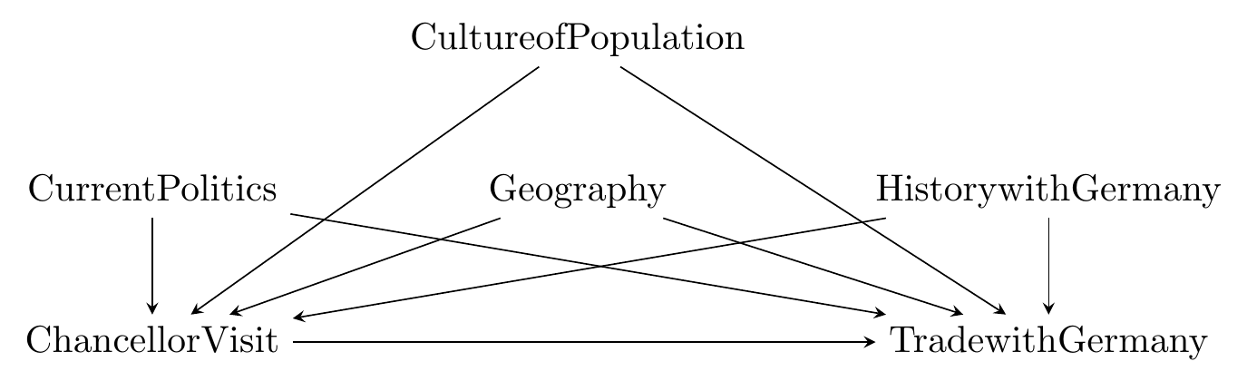
In the diagram, there are quite a few causes of trade with Germany, many of which would be difficult to keep track of or even measure. However, we can also note that several of these variables - the country’s geography, the culture of the population, and the history that country has with Germany - are constant within country or at least (like the culture of the population) are not likely to change much within the span of any data we have.^[“The span of any data you have” is relevant! The longer a time frame your data covers, the more likely it is that some sorta-fixed variable, like geography, is not actually fixed. For example, the geographic borders of Germany have been constant for a long time, but they did vary quite a bit in the 1930s and 1940s. When considering whether a variable is constant over time, it’s really more important to consider whether it’s constant over the time span your data covers.} So we can redraw the diagram as in Figure 16.2.
Figure 16.2: Simplified Causes of Trade with Germany
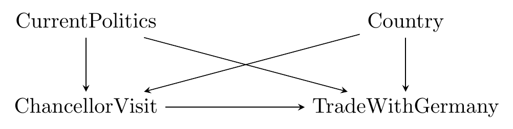
Now, with our simplified figure, we can identify the effect without needing to control for each of the variables in Figure 16.1. We can just control for country instead.449 This logic leads some people to conclude that you can’t identify any effect without having access to some sort of panel data / repeated measurement over time so you can use within variation. But that’s not true! There are plenty of methods in this book that work fine without it. That’s why we worked so hard on writing out our causal diagrams - so we’d know if we needed something like fixed effects.
Keep in mind that we haven’t collapsed everything into country. Anything likely to change regularly over time, like the current politics of a country, won’t be addressed by fixed effects. So if we wanted to identify this effect, we’d still need to control for CurrentPolitics in addition to fixed effects for country.
16.1.2 The Variation Within
Fixed effects, in essence, controls for individual, whether “individual” in your context means “person,” “company,” “school,” or “country,” and so on.450 More broadly, it controls for group at some level of hierarchy. But for simplicity let’s say individual.
What this means is that it gets rid of any variation between individuals. We know that because that’s what it means to control for individual. We’re taking all the variation in our data explained by individual (i.e., all the variation between individuals) and getting rid of it.
Within variation. Variation of a variable that occurs within an individual across (usually) different periods of time.
What’s left is variation within individual. What is variation within individual? For example, let’s say you’re a fairly tall person and we’re tracking your height over time. The fact that you’re taller than other people is between variation. Comparing you to someone else, you’re generally taller. However, we also can observe that, as you grew up from a child to an adult, your height changed over time. Comparing you to your shorter, younger self is within variation. Something changed within individual and that’s what we’re picking up.
Between variation. Variation of a variable that occurs between different individuals, usually at the same period of time, or comparing over-time averages.
The idea of fixed effects is that by sweeping away all that variation between individuals, we’ve controlled for any variables that are fixed over time.451 Technically the effect of those variables must also be fixed over time for this to work, too. For example, no matter where I move in life, I will always have been born in the same city.452 Holler to Arcata, California. Not Arcadia. Easy to mix up. The same goes for everybody else. So all the variation in “city of birth” is between variation. If we get rid of all between variation, we’ve gotten rid of all variation in city of birth, thus controlling for it.
One thing to note about this is that we really have gotten rid of that between variation. So if between variation is what we’re interested in - say, we want to know the effect of city of birth - we can’t do that with fixed effects.453 We can do that with random effects - see later in the chapter.
Let’s walk through two technical examples of this, one with tables and one with graphs. Let’s say we’re interested in the effect of exercise on the number of times a year you get a cold. For subjects in our study, we have you and me. We also suspect there are some variables like “genetics” that are fixed over time that we can adjust for with fixed effects. Let’s start by looking at the data we have on exercise.
Table 16.1: Exercise and Colds
| Individual | Year | Exercise |
|---|---|---|
| You | 2019 | 5 |
| You | 2020 | 7 |
| Me | 2019 | 4 |
| Me | 2020 | 3 |
Table 16.1 shows our raw data, with exercise measured in hours per week. To get our within and between variation, we’ll need to get the within-individual means, shown in Table 16.2.
Table 16.2: Exercise with Within Variation
| Individual | Year | Exercise | MeanExercise | WithinExercise |
|---|---|---|---|---|
| You | 2019 | 5 | 6.0 | -1.0 |
| You | 2020 | 7 | 6.0 | 1.0 |
| Me | 2019 | 4 | 3.5 | 0.5 |
| Me | 2020 | 3 | 3.5 | -0.5 |
Table 16.2 shows how we can take the mean of exercise for each individual, and then subtract out that mean. The difference between individuals in the means is the between variation. So the between variation for exercise comes from comparing your average 6 hours per week against my 3.5 hours per week.
If we subtract out those individual means, we’re left with the way in which we vary from time period to time period relative to our own averages. This is the within variation, looking at how things vary within individual. So my within variation in exercise compares the fact that in 2019 I exercised half an hour per week more than average, and in 2020 I exercised half and hour per week less than average.
We can see this graphically as well. The top-left of Figure 16.3 shows what the data might look like if we gathered it for a few more years.
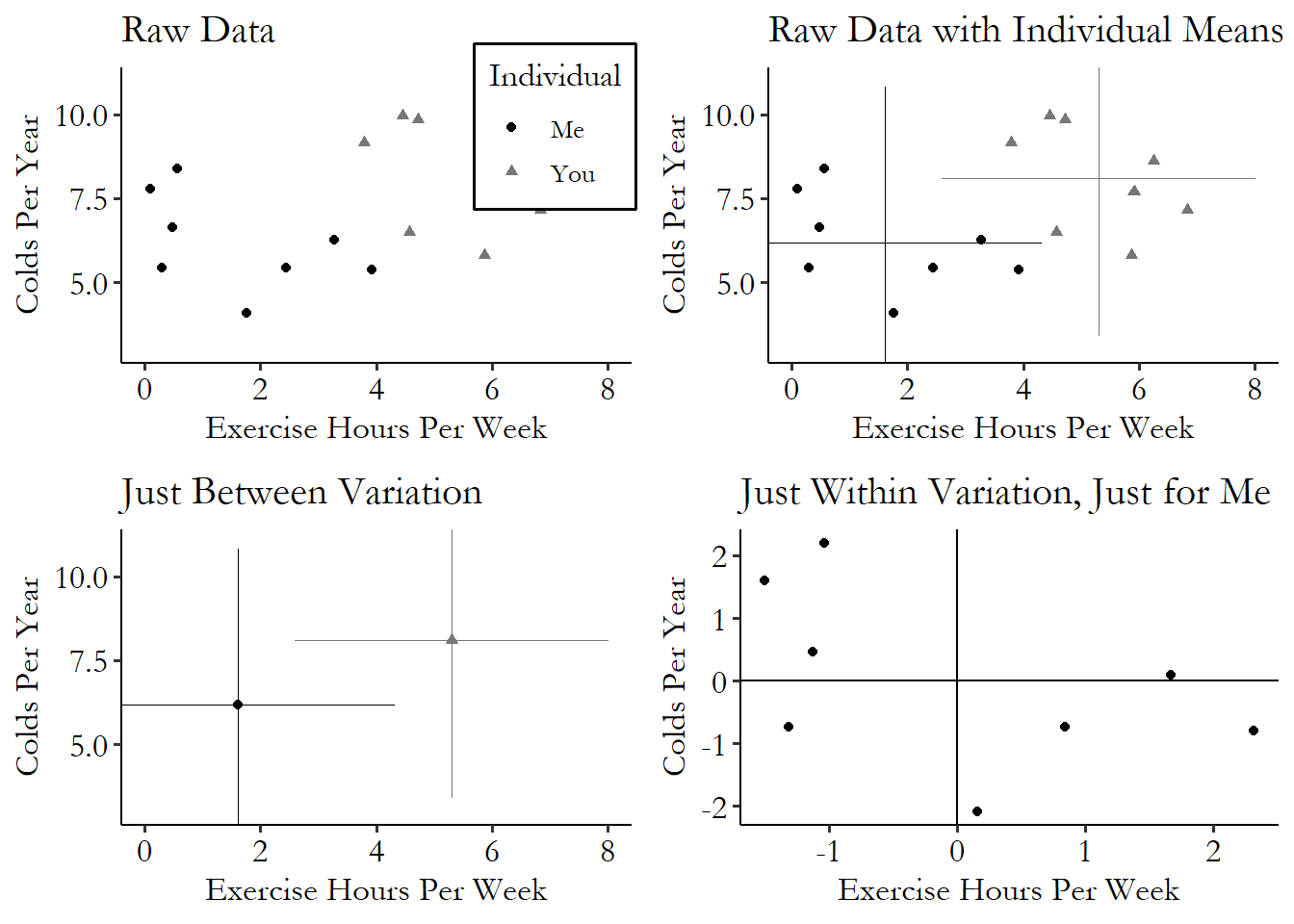
Figure 16.3: Fictional data on exercise per week and number of colds per year for You and for Me, showing how we can isolate between variation by taking You- and Me-specific means, and within variation by subtracting those means out
The top-right takes that raw data and adds some individual-level means. Sort of like each of us is getting their own set of axes. We find the mean exercise and mean number of colds for you, and draw your set of axes at that point. That’s \((0,0)\) on your graph. Similarly, we draw my set of axes where my means are. That’s \((0,0)\) on my graph. Of course, on our shared graph, it’s not \((0,0)\) for anyone, it’s our individual means on both the \(x\)- and \(y\)-axes.
The bottom-left looks just at those axes. We put a point at the center of those axes and ignore everything but those individual means. If we then compare them, say, by drawing a line from one to the other, then we’re looking at the between variation.
In the bottom-right, we forget about you for a second, and just focus on me.454 Try this line on a first date sometime. We zoom in to my set of axes and call those axes \((0,0)\). Now we can see that everything is relative to my own mean. Take that point in the bottom-left, for example. In the top-right graph, that point was about .3 exercise hours per week and about 5.5 colds per year. But in this bottom-right graph, everything is relative to my mean. So instead of .3 and 5.5, it’s about 1.3 fewer hours of exercise per week than my average, and about .8 fewer colds per year than my average.
To actually perform fixed effects, we’d then take your set of axes and slide it over on top of mine! Let’s see how that works.
16.1.3 Fixed Effects in Action
What does fixed effects actually do to data? Well, it’s largely the same as controlling for a categorical variable as described in Chapter 13. We’re isolating within variation. So we find the mean differences between groups (individuals) and subtract them out. That’s basically it.
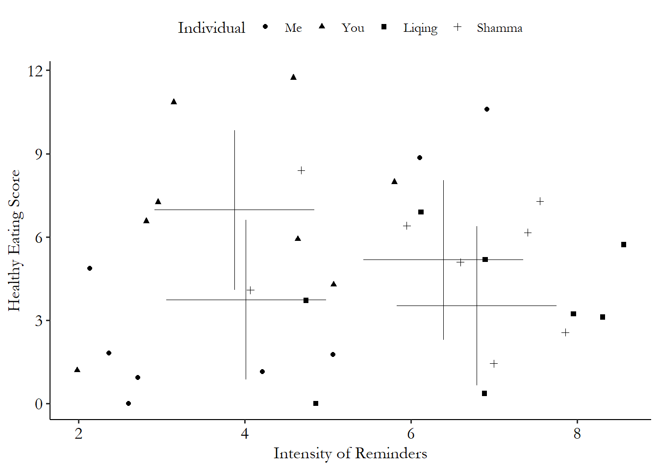
We begin in Figure 16.4 with our raw data, noting that we have several individuals in there. In particular, we are interested in the effects of healthy-eating reminders on actual healthy eating. Our four subjects have each downloaded an app that, at random times, reminds them to eat healthy. They’ve each chosen how frequently they want reminders, but don’t control exactly on which days they come. We’ve recorded how often they get reminders, and also scored them on how healthy they actually eat.
So we have variation over time in how intensively each individual gets reminders, and variation in their healthy eating. There might be some individual-level back doors that led them to choose their frequency and also their general healthy-eating level, so we will want to use fixed effects to close those back doors.
Figure 16.4: Healthy Eating Reminders and Healthy Eating for Four Individuals
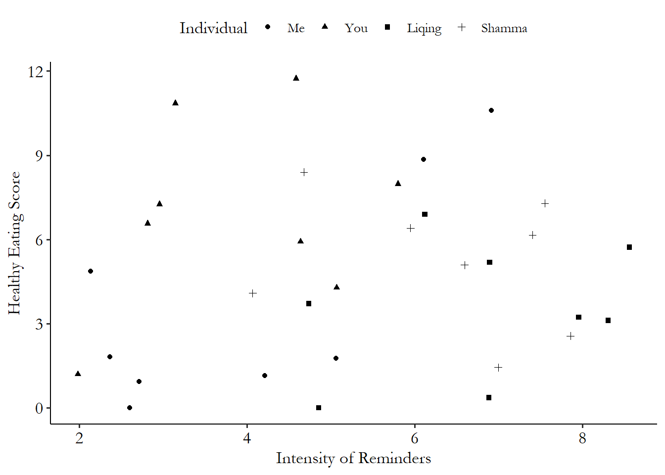
In Figure 16.4 there’s a small positive correlation of .111 between reminders and healthy eating - more reminders means eating healthier! Maybe the messages are effective, if only a tiny little bit.455 Although, looking at the graph itself, this isn’t the most convincing finding. But of course, we haven’t identified the answer to our question yet, since we know there are individual-based back doors. So we start our fixed effects estimation by calculating the mean reminders and mean healthy eating scores for each of our individuals.
Figure 16.5 shows the individual means. There’s clearly a negative relationship between reminders and healthy eating for the individual means. If you just look at the big crosses, they seem to follow a downward slope. The between part of the relationship is negative - the people who choose more frequent messages are the people who tend to eat more poorly on average. The between correlation is -.440.
Figure 16.5: Healthy Eating Reminders and Healthy Eating for Four Individuals
Our next task is to remove any variation between individuals. So we’re effectively going to take all four of those +‘s and slide them on top of each other. First let’s zoom in on each of the four individuals’ within-variation alone, in Figure 16.6.
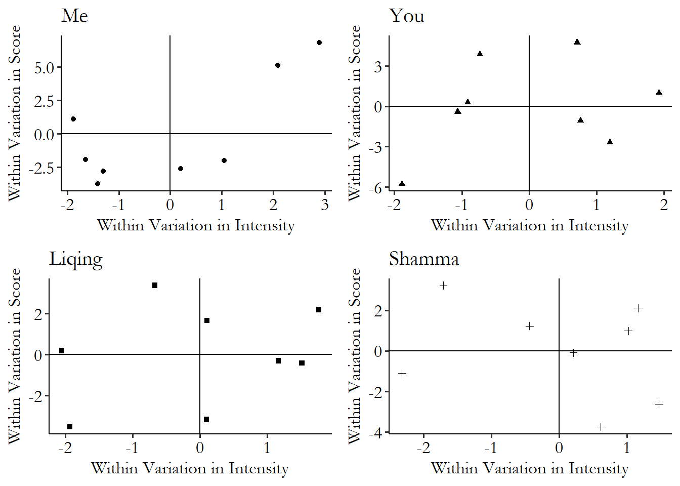
Figure 16.6: Healthy Eating Reminders and Healthy Eating for Four Individuals
Notice that for each of the four graphs in Figure 16.6, the data is centered at 0 on both the \(x\)- and \(y\)-axes. So now when we put all four on top of each other, they’ll be hanging around the same part of the graph.
We put them all on top of each other, aligning all the +’s, in Figure 16.7.
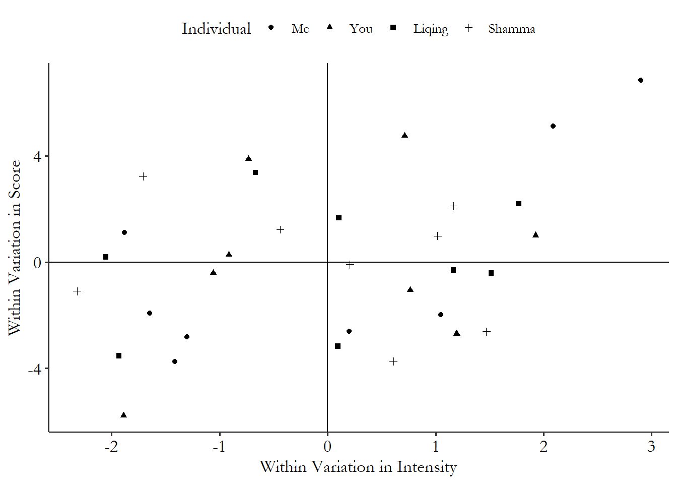
Figure 16.7: Healthy Eating Reminders and Healthy Eating for Four Individuals
Now, with the different individuals moved on top of each other, we see a more clear picture emerging, with a positive relationship between the intensity of reminders and the scores. While the correlation in the raw data was very small, the correlation in the within variation is .363. Much more positive.456 Although still nothing to write home about. I doubt this reminder app is about to get a flurry of interested investors. And since I created this data generating process myself, I can tell you that a positive relationship is indeed correct.
16.2 How Is It Performed?
16.2.1 Regression Estimators
Fixed effects regressions generally start with a regression equation that looks like this:
This looks exactly like our standard regression equation from Chapter 13 with two main exceptions. The first is that \(X\) has the subscript \(it\), indicating that the data varies both between individuals (\(i\)) and over time (\(t\)).
The second is that the intercept term \(\beta\) now has a subscript \(i\) instead of an 0, making it \(\beta_i\). Thinking of regression as a way of fitting a straight line, this means that all the individuals in the data are constrained to have the same slope (there’s no \(i\) subscript on \(\beta_1\)), but they have different intercepts.
Varying intercepts. A regression model in which, even if the slope (coefficient) on each independent variable is restricted to be the same for everyone, the intercept (constant term) is allowed to be different for each individual.
Three obvious questions arise.
QUESTION 1. How does allowing the intercept to vary give you a fixed effects estimate where you use only within variation?
There are two ways to think about this intuitively. The first is procedural. By allowing the intercept to vary, it’s sort of like we’re adding a control for each person. Let’s take a study of countries for example. If India is in our sample, then one of the intercepts is \(\beta_{India}\). This intercept only applies to India, not to any of the other countries.
That’s a lot like adding a “This is India” binary control variable to our regression, and \(\beta_{India}\) is the coefficient on that control variable. We have one of these controls for each country in our data. So we’re controlling for each different country. And we know what happens when we control for country. We get within-country variation.
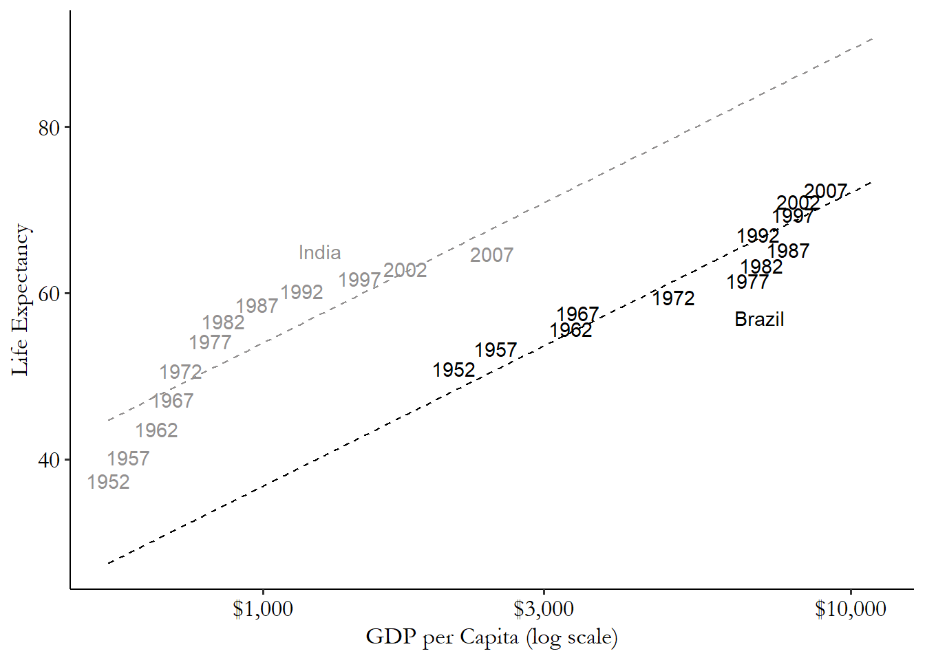
The second way to think about why this works intuitively is to think in terms of a graph. Figure 16.8 uses data on GDP per capita and life expectancy from the Gapminder Institute (Gapminder Institute 2020Gapminder Institute. 2020. “Gapminder.” https://www.gapminder.org/.). Here we’ve isolated just two countries - India and Brazil - and are looking at their data since 1952.
Figure 16.8: GDP per Capita and Life Expectancy in Two Countries
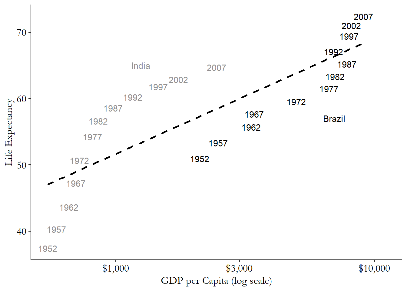
We can see a few things clearly in Figure 16.8. First, things in both countries are clearly getting better over time.457 Neat! However, there are also some clear between-country differences we want to get rid of. And that regression line, with a single intercept for both, is clearly underestimating the slope of the lines that each of the two of them has.
By breaking up the intercept, we can instead use two lines - parallel lines, since they have the same slope - and move them up and down until we hit each country. This lets us not care how far up or down each country’s cluster of points is since we can just move up and down to hit it (we get within variation in the \(y\)-axis variable), and also lets us not care how far left or right each country’s cluster is, since by moving up and down, the same slope can hit the cluster no matter how far out to the right it is (we get within variation in the \(x\)-axis variable). And thus we have within variation.
Figure 16.9: GDP per Capita and Life Expectancy in Two Countries
We do exactly this - the same slope but with different intercepts - in Figure 16.9. The lines are a lot closer to those points now. Those lines capture the relationship that’s clearly there a lot better than the single regression line did.
QUESTION 2. How do we estimate a regression with individual intercepts?
There are actually a bunch of ways to do this. Some of them we will cover in later parts of this chapter.458 Some of them don’t even isolate only the within-variation. Scandalous! But within that long list of ways, there are two standard methods, both of which are dead-simple and only use tools we already know.
The first method is just to extract the within variation ourselves, and work with that.459 This approach gets way trickier if you have more than one set of fixed effects. Just calculate the mean of the dependent variable for each individual (\(\bar{Y}_i\)) and subtract that mean out (\(Y_{it}-\bar{Y}_i\)). Then do the same for each of the independent variables (\(X_{it}-\bar{X}_i\)). Then run the regression
This method is known as “absorbing the fixed effect.”460 \(\beta_0\) is sometimes left out of the equation when doing this method, because it will be 0 anyway. Think about why that should be. Let’s run this approach using the Gapminder data once again.
R Code
library(tidyverse); library(modelsummary)
gm <- causaldata::gapminder

gm <- gm %>%
    # Put GDP per capita in log format since it's very skewed
    mutate(log_GDPperCap = log(gdpPercap)) %>%
    # Perform each calculation by group
    group_by(country) %>%
    # Get within variation by subtracting out the mean
    mutate(lifeExp_within = lifeExp - mean(lifeExp),
    log_GDPperCap_within = log_GDPperCap - mean(log_GDPperCap)) %>%
    # We no longer need the grouping
    ungroup()

# Analyze the within variation
m1 <- lm(lifeExp_within ~ log_GDPperCap_within, data = gm)
msummary(m1, stars = c('*' = .1, '**' = .05, '***' = .01))
Stata Code
causaldata gapminder.dta, use clear download

* Get log GDP per capita since GDP per capita is very skewed
g logGDPpercap = log(gdppercap)

* Get mean life expectancy and log GDP per capita by country
by country, sort: egen lifeexp_mean = mean(lifeexp)
by country, sort: egen logGDPpercap_mean = mean(logGDPpercap)

* Subtract out that mean to get within variation
g lifeexp_within = lifeexp - lifeexp_mean
g logGDPpercap_within = logGDPpercap - logGDPpercap_mean

* Analyze the within variation
regress lifeexp_within logGDPpercap_within
Python Code
import numpy as np
import statsmodels.formula.api as smf
from causaldata import gapminder
gm = gapminder.load_pandas().data

# Put GDP per capita in log format since it's very skewed
gm['logGDPpercap'] = np.log(gm['gdpPercap'])

# Use groupby to perform calculations by group
# Then use transform to subtract each variable's
# within-group mean to get within variation
gm[['logGDPpercap_within','lifeExp_within']] = (gm.
groupby('country')[['logGDPpercap','lifeExp']].
transform(lambda x: x - np.mean(x)))

# Analyze the within variation
m1 = smf.ols(formula = 'lifeExp_within ~ logGDPpercap_within',
data = gm).fit()
m1.summary()
The second simple method is to add a binary control variable for every country (individual). Or rather, every country except one - if our model also has an intercept/constant in it, then including every country will make the model impossible to estimate, so we leave one out, or leave the intercept out.461 Why? Imagine we just have two people - me and you - and are estimating height. Say my average height over time is 66 inches and yours is 68, and we don’t leave anyone out so we have \(Height_{it} = \beta_0 + \beta_1Me_i + \beta_2You_i\). The values \(\beta_0 = 0, \beta_1 = 66, \beta_2 = 68\) gives exactly the same fit as \(\beta_0 = 1, \beta_1 = 65, \beta_2 = 67\). There are infinite ways to get the exact same fit. There’s no way it can choose! So the model can’t be estimated. That one left-out country is still in the analysis; it just doesn’t get its own coefficient. It’s stuck with the lousy constant. Thankfully, most software will do this automatically.
I should point out that this is rarely the way you want to go. Including a set of binary indicators in the model is fine when you have a few different categories, but if you’re controlling for each individual, you may have hundreds or thousands of terms. This can get very, very slow. And c’mon, were you really going to interpret all those coefficients anyway? One common reason to run things this way is so you can do a test of joint significance to see if you even have evidence that there are varying intercepts (see the stuff on the “joint F-test” in Chapter 13). Still, this won’t be your usual go-to for estimating fixed effects. But for demonstrative purposes, we’ll run this version to see what we get.
R Code
library(tidyverse); library(modelsummary)
gm <- causaldata::gapminder

# Simply include a factor variable in the model to get it turned
# to binary variables. You can use factor() to ensure it's done.
m2 <- lm(lifeExp ~ factor(country) + log(gdpPercap), data = gm)
msummary(m2, stars = c('*' = .1, '**' = .05, '***' = .01))
Stata Code
Python Code
import numpy as np
import statsmodels.formula.api as smf
from causaldata import gapminder
gm = gapminder.load_pandas().data
gm['logGDPpercap'] = np.log(gm['gdpPercap'])

# Use C() to include binary variables for a categorical variable
m2 = smf.ols(formula = '''lifeExp ~ logGDPpercap +
C(country)''', data = gm).fit()
m2.summary()
Let’s take a look at our results from the two methods, using the R output, in Table 16.3. With our second method we also estimated a bunch of country coefficients, but those aren’t on the table (there are a lot of them).
| Life Expectancy (within) | Life Expectancy | |
|---|---|---|
| Log GDP per Capita (within) | 9.769*** | |
| (0.284) | ||
| Log GDP per Capita | 9.769*** | |
| (0.297) | ||
| Num.Obs. | 1704 | 1704 |
| R2 | 0.410 | 0.846 |
| RMSE | 5.06 | 5.06 |
| * p < 0.1, ** p < 0.05, *** p < 0.01 |
There are some minor differences between the two in terms of their standard errors, and some big differences in \(R^2\), but the coefficients are the same.462 These code snippets are designed to be illustrative to show how both methods are equivalent. Most of the time, researchers will actually use one of the commands shown in the “Multiple Sets of Fixed Effects” section below, even if they only have one set of fixed effects. So now that we have the coefficients, how can we interpret them?
QUESTION 3. How do we interpret the results of this regression once we have estimated it?
The interpretation of the slope coefficient in a fixed effects model is the same as when you control for any other variable - within the same value of country, how is variation in log GDP per capita related to variation in life expectancy?
Put another way, since we have a coefficient of 9.769, we can say that for a given country, in a year where log GDP per capita is one unit higher than it typically is for that country, then we’d expect life expectancy to be 9.769 years longer than it typically is for that country.463 As you’ll recall from Chapter 13, a one-unit increase in log GDP per capita is a percentage increase in GDP per capita. Specifically, a 171% increase. But for smaller increases, the value and percentage are very close, so we might more often say a log GDP per capita .1 above the typical level, or GDP per capita roughly 10% above, is associated with a life expectancy of .9769 years above the typical level.
What else do we have on the table?
We can see that the \(R^2\) values are quite different in the two columns. Why is this?
Within \(R^2\) One minus the proportion of variance in the residuals relative to the variance in the dependent variable’s within variation.
Remember that \(R^2\) is a measure based on how much variation there is in our residuals relative to our dependent variable.464 \(R^2 = 1 -\) var(residuals) / var(dependent variable), where var is short for variance. In the first column, our dependent variable is \(lifeExp\_within\), not \(lifeExp\). So the \(R^2\) is based on how much variation there is in the residuals relative to the within variation, not the overall variation in \(lifeExp\). This is called the “within \(R^2\).” On the other ahnd, the second column tells us how much variation there is in (those very same) residuals relative to all the variation in \(lifeExp\). It counts the parts of \(lifeExp\) explained by between variation (our binary variables).
Lastly, let’s think about something that’s not on the table - the fixed effects themselves. That is, those coefficients on the country binary variables we got in the second regression. For example, India’s is 13.971 and Brazil’s is 6.318. These are the intercepts in the country-specific fitted lines, like in Figure 16.9.
What can we make of these fixed effects? Not too much in absolute terms,465 We can’t consider them independently because they’re all defined relative to whichever country didn’t get its own coefficient - remember that? So Brazil’s 6.318 doesn’t mean its intercept is 6.318, it means its intercept is 6.318 higher than the intercept of the country that was left out. but they make sense relative to each other. So India’s intercept is \(13.971 - 6.318 = 7.653\) higher than Brazil’s.
We can interpret that to mean that, if India and Brazil had the same GDP per capita, we’d predict that India’s life expectancy would be 7.653 higher than Brazil’s. We’re still looking at the effect of one variable controlling for another - just now, we’re looking at the effect of country controlling for GDP per capita rather than the other way around.
Sometimes researchers will use these fixed effects estimates to make claims about the individuals being evaluated. They might say, for example, that India has especially high life expectancy given its level of GDP per capita.
This can be an interesting way to look at differences between individuals. However, keep in mind that fixed effects is a good way of controlling for a long list of unobserved variables that are fixed over time to look at the effect of a few time-varying variables. Those individual effects don’t have the same luxury of controlling for a bunch of unobserved time-varying variables. We can rarely think of these individual fixed effects estimates as causal.466 In addition, individual fixed effects estimates are estimated based on a relatively small number of observations - just the number we have per individual. So they tend to be a little wild and vary too much. Random effects - discussed later in the chapter - addresses this problem by “shrinkage” of the individual effects.
One last thing to keep in mind about fixed effects. It focuses on within variation. So the treatment effect (Chapter 10) estimated will focus a lot more heavily on people with a lot of within variation. In that life expectancy and GDP example, the coefficient on GDP we got is closer to estimating the effect of GDP on life expectancy in countries where GDP changed a lot over time. If your GDP was fairly constant, you count less for the estimate! You can address this by using weights to address the problem.467 The Gibbons, Suárez, and Urbancic (2019Gibbons, Charles E., Serrato Juan Carlos Suárez, and Michael B. Urbancic. 2019. “Broken or Fixed Effects?” Journal of Econometric Methods 8 (1): 1–12.) paper suggests two solutions, the simplest of which is to calculate the variance of the treatment variable within individual, and weight by the inverse of that. This is an inverse variance weight, like in Chapter 13.
16.2.2 Multiple Sets of Fixed Effects
We’ve discussed fixed effects as being a way of controlling for a categorical variable. This ends up giving us the variation that occurs within that variable. So if we have fixed effects for individual, we are comparing that individual to themselves over time. And if we have fixed effects for city, we are comparing individuals in that city only to other individuals in that city.
So why not include multiple sets of fixed effects? Say we observe the same individuals over multiple years. We could include fixed effects for individual - comparing individuals to themselves at different periods of time, or fixed effects for year - comparing individuals to each other at the same period of time. What if we include fixed effects for both individual and year?
Two-way fixed effects. A model that includes fixed effects for both individual and for year.
This approach - including fixed effects for both individual and for time period - is a common application of multiple sets of fixed effects, and is commonly known as two-way fixed effects. The regression model for two-way fixed effects looks like:
What does this get us? Well, we are looking at variation within individual as well as within year at this point. So we can think of the variation that’s left as being variation relative to what we’d expect given that individual, and given that year.468 Crucially, this is not the same as given that individual that year, as we only observe that individual in that year once. There’s no variation. Each “relative to”s is one at a time.
For example, let’s say we have data on how much each person earns per year (\(Y_{it}\)), and we also have data on how many hours of training they received that year (\(X_{it}\)). We want to know the effect of experience of in-job training on pay at that job.
We do happen to know that the year 2009 was a particularly bad year for earnings, what with the Great Recession and all. Let’s say that earnings in 2009 were $10,000 below what they normally are. And let’s say that we’re looking at Anthony, who happens to earn $120,000 per year, a lot more money than the average person ($40,000).
In 2009 Anthony only earned $116,000. That’s way above average, but that can be explained by the fact that it’s Anthony, and Anthony earns a lot. So given that it’s Anthony, it’s $4,000 below average. But given that it’s 2009, most people are earning $10,000 less, but Anthony is only earning $4,000 less. So given that it’s Anthony, and given that it’s 2009, Anthony in 2009 is earning $6,000 more than you’d expect.
Or at least that’s a rough explanation. Two-way fixed effects actually gets a fair amount more complex than that, since the individual fixed effects affect the year fixed effects and vice versa. Just like with one set of fixed effects, the variation that actually ends up getting used to estimate the treatment effect (Chapter 10) focuses more heavily on individuals that have a lot of variation over time. So if Anthony’s level of in-job training is pretty steady over time, but some other person, Kamala, has a level of training that changes a lot from year to year, then the two-way fixed effects estimate will represent Kamala’s treatment effect a lot more than Anthony’s (De Chaisemartin and d’Haultfoeuille 2020De Chaisemartin, Clément, and Xavier d’Haultfoeuille. 2020. “Two-Way Fixed Effects Estimators with Heterogeneous Treatment Effects.” American Economic Review 110 (9): 2964–96.).
Two-way fixed effects, with individual and time as the fixed effects, aren’t the only way to have multiple sets of fixed effects, of course. As described above, for example, you could have fixed effects for individual and also for city. Neither of those is time!
The interpretation here is a lot closer to thinking of just including controls for individual and controls for city.
One thing to remember, though: we’re isolating variation within individual and also within city. So in order for you to have any variation at all to be included, you need to show up in multiple cities. This is a more common problem here (two sets of fixed effects, neither of them is time) than with two-way fixed effects (individual and time), since generally each person shows up in each time period only once anyway.
If we ran our income-and-job-training study with individual and city fixed effects, the treatment effect would only be based on people and cities which see variation in treatment over time. A given person or city is always treated? It doesn’t count!
Estimating a model with multiple fixed effects can be done using the same “binary controls” approach as for the regular (“one-way”) fixed effects estimator with only one set of fixed effects. No problem!
However, this can be difficult if there are lots of different fixed effects to estimate. The computational problem gets thorny real fast. Unless your fixed effects only have a few categories each (say, fixed effects for left- or right-handedness and for eye color), it’s generally advised that you use a command specifically designed to handle multiple sets of fixed effects.
These methods usually use something called alternating projections, which is sort of like our original method of calculating within variation and using that, except that it manages to take into account the way that the first set of fixed effects gives you within-variation in the other set, and vice versa.
Let’s code this up, continuing with our Gapminder data.
R Code
library(tidyverse); library(modelsummary); library(fixest)
gm <- causaldata::gapminder

# Run our two-way fixed effects model (TWFE).
# First the non-fixed effects part of the model
# Then a |, then the fixed effects we want
twfe <- feols(lifeExp ~ log(gdpPercap) | country + year,
             data = gm)
# Note that standard errors will be clustered by the first
# fixed effect by default. Set se = 'standard' to not do this
msummary(twfe, stars = c('*' = .1, '**' = .05, '***' = .01))
Stata Code
Python Code
import linearmodels as lm
from causaldata import gapminder
gm = gapminder.load_pandas().data
gm['logGDPpercap'] = np.log(gm['gdpPercap'])

# Set our individual and time (index) for our data
gm = gm.set_index(['country','year'])

# Specify the regression model
# And estimate with both sets of fixed effects
# EntityEffects and TimeEffects
# (this function can't handle more than two)
mod = lm.PanelOLS.from_formula(
'''lifeExp ~ logGDPpercap +
             EntityEffects +
             TimeEffects''',gm)

twfe = mod.fit()
print(twfe)
16.2.3 Random Effects
As a research design, fixed effects is all about isolating within variation. We think that there are some back doors floating around in that between variation, so we get rid of it and focus on the within variation. But as a statistical method, fixed effects can really be thought of as a model in which the intercept varies freely across individuals. As I’ve put it before, here’s the model:
It turns out that fixed effects is, statistically, a relatively weak way of letting that intercept vary. After all, we’re only allowing within variation. And how many observations per individual do we really have? We may be estimating those \(\beta_i\)s with only a few observations, making them noisy, which in turn could make our estimate of \(\beta_1\) noisy too.
Random effects takes a slightly different approach. Instead of letting the \(\beta_i\)s be anything, it puts some structure on them. Specifically, it assumes that the \(\beta_i\)s come from a known random distribution, for example assuming that the \(\beta_i\)s follow a normal distribution.
This does a few things:
- It makes estimates more precise (lowers the standard errors).
- It improves the estimation of the individual \(\beta_i\) effects themselves.469 Why? Because we assume that they come from the same distribution. We can use all the data to estimate that distribution, which means each estimate of \(\beta_i\) gets a lot more information to work off of.
- Instead of just using within variation, it uses a weighted average of within and between variation.
- It solves the same back door problem that fixed effects does if the \(\beta_i\) terms are unrelated to the right-hand side variables \(X_{it}\).
That last item is a bit of a doozy. Sure, better statistical precision is nice. But we’re only doing fixed effects in the first place to solve our research design problem. Random effects only solves the same problem if the individual fixed effects are unrelated to our right-hand side variable, including our treatment variable.
That seems unlikely. Consider our Gapminder example. For random effects to be appropriate, the “country effect” would need to be unrelated to GDP. That is, all the stuff about a country that’s fixed over time and determines its life expectancy other than GDP per capita needs to be completely unrelated to GDP per capita. And that list would include things like industrial development and geography. Those seem likely to be related to GDP per capita.
For this reason, fixed effects is almost always preferred to random effects,470 Or at least this version of random effects… keep reading. except when you can be pretty sure that the right-hand side variables are unrelated to the individual effect. For example, when you’ve run a randomized experiment, \(X_{it}\) is a truly randomly-assigned experimental variable and so is unrelated to any individual effect.
One common way around this problem is the use of the Durbin-Wu-Hausman test. The Durbin-Wu-Hausman test is a broad set of tests that compare the estimates in one model against the estimates in another and sees if they are different. In the context of fixed effects and random effects, if the estimates are found to not be different (you fail to reject the null hypothesis that they’re the same), then the relationship between \(\beta_i\) and \(X_{it}\) probably isn’t too strong, so you can go ahead and use random effects with its nice statistical properties.
However, I do not recommend the use of the Durbin-Wu-Hausman test for this purpose.471 I do not like this testing plan. I do not like it, Jerr Hausman. For one thing, if we don’t have a strong theoretical reason to believe that the unrelated-\(\beta_i\)-and-\(X_{it}\) assumption holds, it’s hard to really believe that failing to reject a null hypothesis can justify it for you.
For another, the Durbin-Wu-Hausman test compares fixed effects to the simplest version of random effects, which doesn’t really use random effects to its full advantage. Most studies that use random effects use them in more useful ways that get around that doozy of an assumption. For that, you’ll want to look at the “Advanced Random Effects” section below.
16.3 How the Pros Do It
16.3.1 Clustered Standard Errors
One of the assumptions of the regression model is that the error terms are independent of each other. That is, the parts of the data generating process for the outcome variable that aren’t in the model are effectively random. This assumption is necessary to correctly calculate the regression’s standard errors.
However, we might imagine that this assumption is a tough sell when it comes to fixed effects. After all, we have multiple observations from the same individual or group. We might expect that some of the parts of the data generating process that are left out are shared across all of that individual or group’s observations, making them correlated with each other, and making the standard errors wrong.
For this reason, it’s not uncommon to hear economists say that you should almost always use clustered standard errors when you use fixed effects,472 See the introduction to clustered standard errors in Chapters 13 and 15. specifically standard errors clustered at the same level as the fixed effect. So for person fixed effects, for example, using standard errors clustered at the person level. Or for city fixed effects, using standard errors clustered at the city level. Clustered standard errors calculate the standard errors while allowing some level of correlation between the error terms.
However, this common wisdom goes a bit too far. For clustering with fixed effects to be necessary (and a good idea), several conditions need to hold. First, there needs to be treatment effect heterogeneity. That is, the treatment effect must be quite different for different individuals.
If that is true, there’s a second condition. Either the fixed effect groups/individuals in your data need to be a nonrandom sampling of the population,473 That is, some groups are more likely to be included in your sample than others. or, within fixed effect groups/individuals, your treatment variable is assigned in a clustered way.474 For example, with city fixed effects, are certain individuals in that city more likely to be treated than others?
So before clustering, think about whether both conditions are likely to be true (Abadie et al. 2023Abadie, Alberto, Susan Athey, Guido W. Imbens, and Jeffrey M. Wooldridge. 2023. “When Should You Adjust Standard Errors for Clustering?” The Quarterly Journal of Economics 138 (1): 1–35.). If it is, go ahead and cluster! If not, don’t bother, as the clustering will make your standard errors larger than they’re supposed to be.
Clustered standard errors usually come packaged with the same commands that are used to perform fixed effects, since people so commonly use clustered errors with fixed effects. Using Gapminder data once again:
R Code
Stata Code
Python Code
import pandas as pd
import linearmodels as lm
from causaldata import gapminder
gm = gapminder.load_pandas().data
gm['logGDPpercap'] = np.log(gm['gdpPercap'])

# Set our individual and time (index) for our data
gm = gm.set_index(['country','year'])

mod = lm.PanelOLS.from_formula(
'''lifeExp ~ logGDPpercap +
              EntityEffects''',gm)

# Specify clustering when we fit the model
clfe = mod.fit(cov_type = 'clustered',
               cluster_entity = True)
print(clfe)
16.3.2 Fixed Effects in Nonlinear Models
The intuition behind the fixed effects research design applies consistently to all sorts of statistical models. We think there’s a back door that can be closed by getting rid of all the between variation, so we do that.
However, the methods we have for getting rid of that variation - adding a set of binary control variables for the fixed effects, or subtracting out the individual means - do not extend to all sorts of statistical models. Both of those approaches assume that we’re using a linear model. That will be a problem if we’re not using a linear model. Perhaps we’re using probit, or logit, or Poisson, or tobit, or ordered logit, and so on and so on.
Why might this be a problem?
First, let’s consider the approach where we include binary control variables. Including a set of binary control variables is fine as long as there aren’t too many of them. For example, fixed effects for left-or-right handedness, or fixed effects for eye color. There aren’t too many variations of those, so including controls for each option isn’t too bad. The problem comes when there are lots of groups, as there might be in many “fixed effects for individual” settings. For example, in our Gapminder analysis there are 142 different countries in the data. This entails adding 142 control variables and estimating 142 coefficients. That’s fine in a linear model, but in a nonlinear model you run into the “incidental parameters problem,” where it just can’t handle estimating that much stuff. The estimates start getting noisy and bad.
Second, let’s consider the version where we subtract out the within-group means. This no longer works because the outcome variable isn’t a continuous variable any more, so the mean is no longer a good representation of “what I need to subtract out to get rid of the between variation.” The intuition still works, but subtracting out the mean is no longer the right trick.
So what can we do? We still might want to use a fixed effects design even if we have a nonlinear dependent variable.
There are two common approaches people take. One is to drop the “nonlinear” part and just estimate a linear model anyway with your nonlinear dependent variable. This is especially common when the dependent variable is binary or ordinal. Many researchers, especially economists, consider the downsides of the misspecified linear model (with heteroskedasticity-robust standard errors) to not be as bad as the downsides associated with trying to estimate an actual nonlinear model with fixed effects.475 This is, unfortunately, a matter of taste. There’s not a single right answer here.
Another common approach is to use a nonlinear model variant that is designed to handle fixed effects properly. Things are likely out of your hands at this point and in the hands of the econometricians. Look for a method (or a software command) designed to do what you need. It might not exist! But if it does, make sure to read the documentation so you understand what you’re doing, and then use that.
There are too many different methods to go into them here, but once you come to this point you are probably down to searching the Internet and reading about your particular application. And keep in mind that there are usually multiple different ways to do this, each of which means something different.
However, the most common applications here are for binary dependent variables and wanting to do probit or logit with fixed effects. In R, look at the generalized linear model options in the fixest package. In Stata use the commands xtprobit, xtlogit, or xtPoisson. In Python there is the pylogit package, which allows you to do conditional logit regression, which is similar but not quite the same.
16.3.3 Advanced Random Effects
In the Random Effects section above, I mentioned that fixed effects is usually preferred to random effects unless you have a strong reason (like randomization) to think that your right-hand side variables are unrelated to the individual effects.
However, this argument uses a bit of a straw-man version of random effects. Lots of researchers use random effects even when the individual effect is almost certainly related to the right-hand side variables. Surely they can’t all be unaware of the problem!
Multi-level model. A model in which the coefficients themselves are allowed to vary over the sample, potentially with other variables explaining how they vary.
And in fact, they are not. Modern approaches to random effects are more than capable of handling this issue (Bell and Jones 2015Bell, Andrew, and Kelvyn Jones. 2015. “Explaining Fixed Effects: Random Effects Modeling of Time-Series Cross-Sectional and Panel Data.” Political Science Research and Methods 3 (1): 133–53.). This generally works by seeing your model as containing multiple levels. This makes sense for the context - in any fixed effects setting our data is hierarchical. At the very least, it has multiple observations over time within individual. The data has levels. Let’s model those levels.
So for example, perhaps we have the model:
That’s one of our levels. We would then say that the \(\beta_i\) term itself follows its own equation:
where \(Z_{i}\) is a set of individual-level variables that determine the individual effect, and \(\mu_i\) is an error term.
This allows us to deal with the correlation between the \(\beta_i\) and the \(X_{it}\) because we’re modeling it directly. That individual-level time-consistent part of \(X_{it}\) that might be related to \(\beta_i\) - hopefully we account for that part of it with the \(Z_{i}\).
This approach does a few nice things for us. First of all, it gets us the nice statistical properties that random effects gives us over fixed effects, but without imposing as many additional assumptions.
Second, it lets us look at the effect of variables that are constant within individual. Let’s say we wanted to look at the effect of hometown on whether you become an inventor. Well, each person’s hometown doesn’t change over their lifetime, so fixed effects would never let us study that question. But multi-level random effects would.
Third, it lets us explicitly look at between and within effects separately. Fixed effects says “within effects only, please.” Basic random effects says “some mix of between and within.” Multi-level random effects, if done properly, says “here are the between effects, and here are the within effects. Do what you will.”
There are two directions we can go with this multi-level intuition in mind.
One approach, which helps explicitly separate out the between and within effects, is just to… include both effects in the regression. Simple as that!476 This descends from, although is not exactly the same as, Mundlak (1978Mundlak, Yair. 1978. “On the Pooling of Time Series and Cross Section Data.” Econometrica 46 (1): 69–85.).
All you do is:
- Calculate within-individual means for each predictor (\(\bar{X}_i\)).
- Calculate the within variation for each predictor (\(X_{it} - \bar{X}_i\)).
- Regress the dependent variable on the within-individual means (\(\bar{X}_i\)), the within variation (\(X_{it} - \bar{X}_i\)), and any other individual-level controls you like (\(Z_i\)), and use random effects for the intercept.
This is referred to as “correlated random effects.” It is handy in that it separates out for you the “between variation effect” (the coefficients on the \(\bar{X}_i\)s) and the “within variation effect” (the coefficients on the \(X_{it} - \bar{X}_i\)s), and also lets you see the effect of individual-level variables \(Z_i\). You wanted that within effect from fixed effects anyway, and now you get some bonus stuff on top.
This approach is easy to implement and easy to interpret. If you can calculate within-individual means and within variation (code in the “How Is It Performed” section), then you can just toss everything into a model with random effects (in R, see lmer in the lme4 package; in Stata see xtreg with the re option; and in Python see RandomEffects in the linearmodels package).
The other way we can go with our multi-level intuition is whole hog into mixed models, also known as hierarchical linear models.
Mixed models say we don’t need to stop at the intercept following a random distribution. Why stop there? How about the slope coefficients on the other variables?
These models can get complex, but they can be used to represent very complex interactions between variables. After all, this is social science. Everything is complex! We might well expect that there are a bunch of variables that don’t just explain \(Y_{it}\), but explain how \(X_{it}\) affects \(Y_{it}\) and we want to model that.
Mixed models are extremely common in many fields, and if you’re from one of those fields you might be surprised to find them tucked away in a little subsection in one chapter of this book. Alas, as the focus of this book is design rather than estimation, it makes sense to talk about fixed effects first and include mixed models as an extension of that.477 I can practically feel the presence of Andrew Gelman reaching through time and space to disagree with this characterization. Maybe the only reason putting mixed models here makes sense to me is I’m an ignorant economist. Sorry, Andrew.
Still, they are worth exploring outside the confines of this book. I recommend the textbook by Gelman and Hill (2006Gelman, Andrew, and Jennifer Hill. 2006. Data Analysis Using Regression and Multilevel/Hierarchical Models. Cambridge University Press.) for further reading. You can also try mixed models out yourself with lmer in the lme4 package in R; xtmixed in Stata; or mixedlm in the statsmodels package in Python. More broadly, there is Stan, which is sort of its own language dedicated entirely to fast and flexible estimation of hierarchical models.478 https://mc-stan.org/ Stan can be used from other languages, and the intuitively-named RStan, StataStan, and PyStan packages are all available.
Page built: 2025-10-17 using R version 4.5.0 (2025-04-11 ucrt)