Chapter 13 - Regression

13.1 The Basics of Regression
Regression is the most common way in which we fit a line to explain variation. Using one variable to explain variation in another is a key part of what we’ve been doing the whole book so far!
When it comes to identifying causal effects, regression is the most common way of estimating the relationship between two variables while controlling for others, allowing you to close back doors with those controls.197 Saying we “adjust” for those variables, rather than control for them, is probably more accurate, since we don’t actually have control of anything here as we would in a controlled experiment. But “control” is the most common way of saying it. Naturally it’s relevant to what we’re doing. Not only will we be discussing it further in this chapter, but many of the methods described in other chapters of Part II of the book are themselves based on regression.
We’ve already covered the basics of regression, back in Chapter 4. So go back and take a look at that.
Some key points from that chapter:
- We can use the values of one variable (\(X\)) to predict the values of another (\(Y\)). We call this explaining \(Y\) using \(X\).198 This is a purely statistical form of “explanation.” It’s not an explanation why \(Y\) happens (unless we’ve identified the effect of \(X\) on \(Y\)), just the ability to predict \(Y\) using \(X\).
- While there are many ways to do this, one is to fit a line or shape that describes the relationship. For example, \(Y = \beta_0 + \beta_1X\). Estimating this line using ordinary least squares (standard, linear regression) will select the line that minimizes the sum of squared residuals, which is what you get if you take the prediction errors from the line, square them, and add them up. Linear regression, for example, gives us the best linear approximation of the relationship between \(X\) and \(Y\). The quality of that approximation depends in part on how linear the true model is.
- Pro: Uses variation efficiently
- Pro: A shape is easy to explain
- Con: We lose some interesting variation
- Con: If we pick a shape that’s wrong for the relationship, our results will be bad
- We can interpret the coefficient that multiplies a variable (\(\beta_1\)) as a slope. So, a one-unit increase in \(X\) is associated with a \(\beta_1\) increase in \(Y\).
- With only one predictor, the estimate of the slope is the covariance of \(X\) and \(Y\) divided by the variance of \(X\). With more than one, the result is sort of similar, but also it accounts for the way the different predictors are correlated.
- If we plug an observation’s predictor variables into an estimated regression, we get a prediction \(\hat{Y}\). This is the part of \(Y\) that is explained by the regression. The difference between \(Y\) and \(\hat{Y}\) is the unexplained part, which is also called the “residual.”
- If we add another variable to the regression equation, such as \(Y = \beta_0 + \beta_1X+ \beta_2Z\), then the coefficient on each variable will be estimated using the variation that remains after removing what is explained by the other variable. So our estimate of \(\beta_1\) would not give the best-fit line between \(Y\) and \(X\), but rather between the part of \(Y\) not explained by \(Z\) and the part of \(X\) not explained by \(Z\). This “controls for \(Z\).”
- If we think the relationship between \(Y\) and \(X\) isn’t well-explained by a straight line, we can use a curvy one instead. Ordinary least squares (OLS) can handle things like \(Y = \beta_0+ \beta_1X + \beta_2X^2\) that are “linear in parameters” (notice that the parameters \(\beta_1\) and \(\beta_2\) are just plain multiplied by a variable, then added up), or we can use nonlinear regression like probit, logit, or a zillion other options.
Those are the basics that more or less explain how regression works. And as long as that regression model looks like the population model (the true relationship is well-described by the shape we choose), it has a good chance of working pretty well. But there’s still plenty left to cover. What else do we need to know?
We’re going to add a few pieces of OLS that we haven’t covered yet, or at least not thoroughly:
- The error term
- Sampling variation
- The statistical properties of OLS
- Interpreting regression results
- Interpreting coefficients on binary and transformed variables
That’s a lot to get through! Let’s get going.
13.1.1 Error Terms
Residual. The difference between a prediction and the actual outcome.
Error. The difference between the actual outcome and prediction we’d make if we had infinite observations to estimate our prediction.
A lot of the detail of regression is hidden in the places it doesn’t go. I previously described fitting a straight line as figuring out the appropriate \(\beta_0\) and \(\beta_1\) values to give us the line \(Y = \beta_0 + \beta_1X\).
However, in our actual data, that line is clearly insufficient. It will rarely predict any observation perfectly, much less all of the observations. There’s going to be a difference between the line that we fit and the observation we get. That’s what I mean by “the places it doesn’t go.” We can add this difference to our actual equation as an “error term” which I’ll mark as \(\varepsilon\). So now our equation is:
That difference goes by two names: the residual, which we’ve talked about, is the difference between the prediction we make with our fitted line and the actual value, and the error is the difference between the true best fit-line and the actual value. Why the distinction? Well… sampling variation. Because we only have a finite sample, the best-fit line we get with the data we have won’t quite be the same as the best-fit line we’d get if we had data on the whole population.199 Remember Chapter 3? All we can really see will be the residual, but we need to keep that error in mind. As we know from Chapter 3, we want to describe the population. Those population-level errors will help us figure out what’s going on.
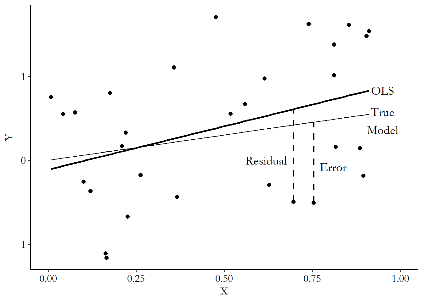
You can see the difference between a residual and an error in Figure 13.1. The two lines on the graph represent the true model that I used to generate the data in the first place, and the OLS best-fit line I estimated using the randomly-generated sample. For each point, the vertical distance from that point to the OLS line is the residual (since the OLS line represents our prediction), and the vertical distance from that point to the true model is the error (since even if we knew the true model relating \(Y\) and \(X\), we still wouldn’t predict the point perfectly because of the other stuff that goes into \(Y\)).
Figure 13.1: The Difference Between the Residual and the Error
So what’s in an error, anyway? Where does it come from? Well, the error effectively contains everything that causes \(Y\) that is not included in the model. \(Y\) is on the left-hand-side of the \(Y = \beta_0 + \beta_1X + \beta_2Z + \varepsilon\) equation, and it’s determined by the right-hand-side. So if there’s something that goes into \(Y\) but isn’t \(X\) or \(Z\), then it has to come from somewhere. That somewhere is \(\varepsilon\).
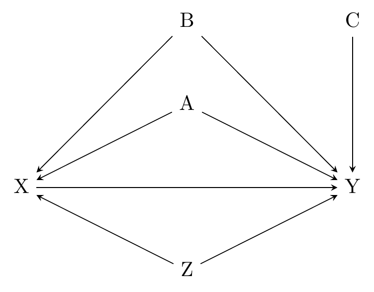
\(\varepsilon\) includes both stuff we can see and stuff we can’t. So, for example, if the true model is given by Figure 13.2, and we are using the OLS model \(Y = \beta_0 + \beta_1X + \beta_2Z + \varepsilon\), then \(\varepsilon\) is made up of some combination of \(A\), \(B\), and \(C\). We know that since we can determine from the graph that \(A\), \(B\), and \(C\) all cause \(Y\), but they aren’t in the model.
Figure 13.2: Depending on the Model Used, A, B, C, and Z Might Be in the Error Term
13.1.2 Regression Assumptions and Sampling Variation
Thinking about what’s in the error term leads us to the first assumption we’ll need to make about the error term. There are going to be a few of these assumptions, and I’ll bring them up as they become necessary. People who use regression tend to be obsessed about those lil’ \(\varepsilon\)s and the assumptions we make about them. Go to any research seminar, and you’ll hear endless questions about error terms and whether the assumptions we need to make about them are likely to be true.
Exogeneity assumption. In a regression context, the assumption that the variables in the model (or perhaps just our treatment variable) are uncorrelated with the error term.
The first assumption we’ll talk about links the first and second parts of the book, and it’s the exogeneity assumption. If we want to say that our OLS estimates of \(\beta_1\) will, on average, give us the population \(\beta_1\), then it must be the case that \(X\) is uncorrelated with \(\varepsilon\).200 Oddly, this does not require that \(X\) and \(\varepsilon\) are completely unrelated, just uncorrelated - there can be a relationship between the two, just not a linear relationship. For example, if the relationship between \(X\) and \(\varepsilon\) looks like a V or a U, then they’re clearly related, but a straight line describing the relationship would be flat. The downward part would cancel out with the upward part. In reality, it’s pretty rare that two variables are related but completely uncorrelated, so this doesn’t usually let us get away with ignoring a relationship between \(X\) and \(\varepsilon\).
If that sounds familiar, it’s because we’re really just restating the conditions for identifying a causal effect! Every variable that causes \(Y\) in a causal diagram like Figure 13.2 ends up in the regression equation somehow, whether it’s one of the variables in the model or just in \(\varepsilon\). If a variable is in the regression equation directly, then that closes any causal paths that go through that variable. By adding a variable to the regression, we “control for it” or “add it as a control.” So with the regression \(Y = \beta_0 + \beta_1X + \beta_2Z + \varepsilon\), the path \(X \leftarrow Z \rightarrow Y\) is closed.
But if something is still in the error term and is correlated with \(X\), we haven’t closed the path. Since \(A\) is in \(\varepsilon\), and we know from the diagram that \(A \rightarrow X\), then we can say either that (a) we haven’t closed the \(X \leftarrow A \rightarrow Y\) back door path, and so the effect of \(X\) isn’t identified, or, (b) \(X\) is correlated with \(\varepsilon\) and so is “endogenous” rather than exogenous, and the effect of \(X\) isn’t identified.201 The terms “endogeneity” and “exogeneity” come from the biology terms “endogeny” and “exogeny,” which roughly mean “from within the system” and “from outside the system.” Endogenous variables are determined by other things in the system (other things that are part of determining the outcome). These are saying, in effect, the same thing, just using lingo from different domains.202 There are yet other ways to talk about this in other fields. You could also say that \(A\) is an “unobserved/unmeasured confounder” or that \(X\) and \(Y\) have a “spurious correlation.”
Similarly, we can say in either set of lingo that we don’t need to worry about \(C\) being in our model. It’s in the error term - everything that predicts \(Y\) but isn’t in the model is in the error term. But we can say either (a) there’s no back door from \(X\) to \(Y\) that goes through \(C\), or (b) \(X\) is unrelated to \(C\) and so \(C\) isn’t leading \(X\) to be endogenous.
Bias. An estimate that, on average, gives the wrong answer, no matter how big your sample size gets, is biased.
Omitted variable bias. Bias in a regression estimate that occurs because a variable correlated with the treatment is in the error term and otherwise omitted from the model.
Speaking of lingo, if we do have that endogeneity problem, then on average our estimate of \(\beta_1\) won’t give us the population value. When that happens - when our estimate on average gives us the wrong answer, we call that a bias in our estimate. In particular, this form of bias, where we are biased because a variable correlated with \(X\) is in the error term, is known as omitted variable bias, since it happens because we omitted an important variable from the regression equation. Previously in the book we’d say we failed to close the back door that goes through \(A\). In this lingo, we’d say that \(A\) gave us omitted variable bias, but \(C\) doesn’t.
So that’s our first assumption about the error term - the exogeneity assumption, that \(\varepsilon\) is uncorrelated with any variable we want to know the causal effect of. We know how to think about whether that assumption is true - the entire first half of this book is about figuring out what’s necessary to identify a causal effect.
Of course, that’s only the first thing we need to assume about the error term. Many of the others, though, relate to the sampling variation of the OLS estimates.
Just like the means we discussed in Chapter 3, regression coefficients are estimates, and even though there’s a true population model out there, the estimate we get varies from sample to sample due to sampling variation.
Conveniently, we have a good idea what that sampling variation looks like. We know that we can think of observations as being pulled from theoretical distributions. We also know that statistics like the mean can also be thought of as being pulled from theoretical distributions. In the case of the mean, that’s a normal distribution (see Chapter 3). If you drew a whole bunch of samples of the population and took the mean each time, the distribution of means across the sample would follow a normal distribution. Then we can use the estimated mean we get to try to figure out what the population mean is.
Regression coefficients also follow a normal distribution, and we know what the mean and standard deviation of that normal distribution is. Or, at least we do if we make a few more assumptions about the error term.
What is that normal distribution that the OLS coefficients follow?203 The following calculations will assume that the exogeneity assumption mentioned earlier holds.
In a regression model with one predictor, like \(Y = \beta_0 + \beta_1X + \varepsilon\), an OLS estimate \(\hat{\beta}_1\) of the true-model population \(\beta_1\) follows a normal distribution with a mean of \(\beta_1\) and a standard deviation of \(\sqrt{\sigma^2/(var(X)n)}\), where \(n\) is the number of observations in the data, \(\sigma\) is the standard deviation of the error term \(\varepsilon\), and \(var(X)\) is the variance of \(X\).204 Wait, how do we get the standard deviation of \(\varepsilon\) if we can’t see it? Well, we don’t know it exactly, so our idea of this sampling distribution will itself be an estimate based on our best guess of \(\sigma\). We use the residual, which we can see, instead of the error, and base our estimate of \(\sigma\) on the standard deviation of the residual. This standard deviation isn’t generally called a standard deviation, though. The standard deviation of a sampling distribution is often referred to as a standard error. And that’s what we’ll call them here too.
Standard error. The standard deviation of a sampling distribution.
If there’s more than one variable in the model, the math starts to require matrix algebra, but it’s the same idea. In the regression model \(Y = \beta_0 + \beta_1X+ \beta_2Z + \varepsilon\), the OLS estimates \(\hat{\beta}_1\) and \(\hat{\beta}_2\) follow a joint normal distribution, where their respective means are the population \(\beta_1\) and \(\beta_2\), and the standard deviations are the square roots of the diagonal of \(\sigma^2(A'A)^{-1}/n\), where \(A\) is a two-column matrix containing both \(X\) and \(Z\). But you can think of \((A'A)^{-1}\) as saying “divide by the variances and covariances of \(X\) and \(Z\),” just like \(\sqrt{\sigma^2/(var(X)n)}\) says “divide by the variance of \(X\).”
How can we make an OLS estimate’s sampling variation really small? There are only three terms in the standard deviation, so only three things to change: (1) We could shrink the standard deviation of the error term \(\sigma\), i.e., make the model predict \(Y\) more accurately, (2) we could pick an \(X\) that varies a lot and has a big variation - an \(X\) that changes a lot makes it easier to check whether \(Y\) is changing at the same time, or (3) we could use a big sample so \(n\) gets big.
How about those other assumptions we need to make about the error term? It turns out that those assumptions are necessary to assume that the stuff I’ve said up to now about the standard error is true. Let’s tuck that away in our back pocket for now and ignore that looming problem. We’ll come back to it in the “Your Standard Errors are Probably Wrong” section below. All of the things I’m going to say now about using standard errors will still hold up. There might just need to be some minor adjustments to the way we calculate them, which is what we’ll discuss in that section.
13.1.3 Hypothesis Testing in OLS
Okay, so why did we want to know the OLS coefficient distribution again? The same reason we want to think about any theoretical distribution - theoretical distributions let us use what we observe to come to the conclusion that certain theoretical distributions are unlikely.
And since the theoretical distribution of our OLS estimate \(\hat{\beta}_1\) is centered around the population parameter \(\beta_1\), that means we can use our estimate \(\hat{\beta}_1\) to say that certain population parameters are very unlikely, for example “it’s unlikely that the effect of \(X\) on \(Y\) is 13.2.”
To recap what we’re doing here, modifying only slightly what we have from Chapter 3:
- We pick a theoretical distribution, specifically a normal distribution centered around a particular value of \(\beta_1\)
- Estimate \(\beta_1\) using OLS in our observed data, getting \(\hat{\beta}_1\)
- Use that theoretical distribution to see how unlikely it would be to get \(\hat{\beta}_1\) if indeed the true population value is what we picked in the first step
- If it’s super unlikely, that initial value we picked is probably wrong!205 Or, if you’re Bayesian, that initial value needs to be revised a lot.
We can take this a step further towards the concept of hypothesis testing. Hypothesis testing is a way of formalizing the four steps above into a way of making a decision about whether we can “reject” the theoretical distribution, and thus the original \(\beta_1\) we picked.206 There are plenty of reasons not to like hypothesis testing, but it’s extremely common, and so you have to know about it to figure out what’s going on. What’s wrong with it? It depends on the arbitrary and strangely sharp choice of rejection value (\(p = .049\) rejects the null, but \(p = .051\) doesn’t?), and it also relies on the idea that you’ve “found a result” when you’ve really just rejected something obviously false. In social science, very few relationships are truly exactly zero, and yet that’s almost always our null-hypothesis value. So with enough sample size we always reject the null. My opinion: use significance testing; it is useful and it helps you converse with other people doing research. But don’t get too serious about it. And certainly never choose your model based on significance! The first half of this book is about much better ways to choose models.
Under hypothesis testing, we pick a “null hypothesis” - the initial \(\beta_1\) value we’re going to check against. In practice, this is almost always zero (although it certainly doesn’t have to be), so let’s simplify and say that our null hypothesis is \(\beta_1 = 0\).
Then, we pick a “rejection value” \(\alpha\). If we calculate that the probability of getting our estimated result from the theoretical distribution based on \(\beta_1 = 0\) is below \(\alpha\), then we say that’s too unlikely, and conclude that \(\beta_1 = 0\) is false, rejecting it. Commonly, this rejection value is \(\alpha = .05\), so if the estimate we get (or something even stranger) has a 5% chance or less of occurring if the null value is true, then we reject the null.
Once we’ve rejected \(\beta_1 = 0\), what conclusion can we come to? Not that our estimate is correct - we certainly don’t know that; there are plenty of nonzero values we haven’t rejected. All we can say is that we don’t think it’s likely to be 0. Knowing it’s not zero can be handy - if it’s not zero, that means there’s some relationship there. And that’s our conclusion.
To see this in action, I generated 200 random observations using the true model \(Y = 3 + .2X + \varepsilon\), where \(\varepsilon\) is normally distributed with mean 0 and variance 1. Then, pretending that we don’t know the truth is \(\beta_1 = .2\), I estimated the OLS model using the regression \(Y = \beta_0 + \beta_1X + \varepsilon\).
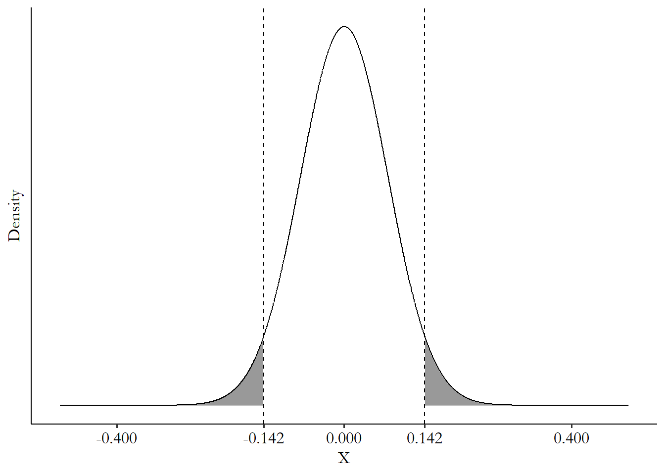
The first estimate I get is \(\hat{\beta_1} = .142\). I can use the formula from the last section to also calculate that the standard error of \(\beta_1\) is \(se(\beta_1) = .077\). So the theoretical distribution I’m looking at is a normal distribution with mean 0 and standard deviation \(.077\).
Under that distribution, the \(.142\) estimate I got is at the 96.7th percentile of the theoretical distribution, as shown in Figure 13.3. That means that something as far from 0 as \(.142\) is (or farther) happens \((100 - 96.7)\times 2 = 3.3\times2 =\) 6.6% of the time.207 Note I’ve doubled the percentile here - that’s because “as far away or farther” includes both sides of the distribution. This is a “two-tailed test,” which is standard. If we did a “one-tailed test,” caring only if it was as far away or farther in the same direction, we wouldn’t do the doubling. If we started with \(\alpha = .05\), then we would not reject the \(\beta_1 = 0\) null hypothesis, since 6.6% is higher than 5%, even though we happen to know for a fact that the null is quite wrong.
Figure 13.3: Comparison of Our .142 Estimate to a Theoretical Null Distribution Centered at 0
We can see how this works from a different angle in Figure 13.4. This time I’m generating a bunch of samples of random data and showing the sampling distribution against a given null value. I’m magically giving myself the knowledge that \(\beta_1 = .2\) is the true value to test against. I generate random data from that same true model \(Y = 3 + .2X + \varepsilon\) a whole bunch of times, estimate \(\hat{\beta}_1\) using OLS, and test it against the null of \(\beta_1 = .2\). Sometimes I still reject the null, even though the null is literally true, but not often. In fact, I reject it exactly 5% of the time, because of the \(\alpha = .05\) decision. Sampling variation will do that! This is a rejection of something that’s true, and how often we do it is the “false positive” rate, or the terribly-named “type I error rate.”208 Why is it a false “positive”? Because we sort of think about hypothesis testing as a “success” when we reject the null. This is silly, of course - we want to find the true value, not just go around rejecting nulls. A well-estimated non-rejection is much more valuable than a rejection of the null from a bad analysis. But there seems to be something in human psychology that makes us not act as though this is true.
I then test those same estimates against the null of \(\beta_1 = 0\). Sometimes I fail to reject the null, even though the null is false. Sampling variation does this too! Our failure to reject false nulls is the “false negative” rate or the “type II error rate.”
What these figures demonstrate is that hypothesis testing really isn’t about pinning down a true value, nor is it about hard-and-fast, true-and-false results. It’s about showing that certain theoretical distributions are unlikely. And we can then say that if they’re too unlikely, we can forget about them.
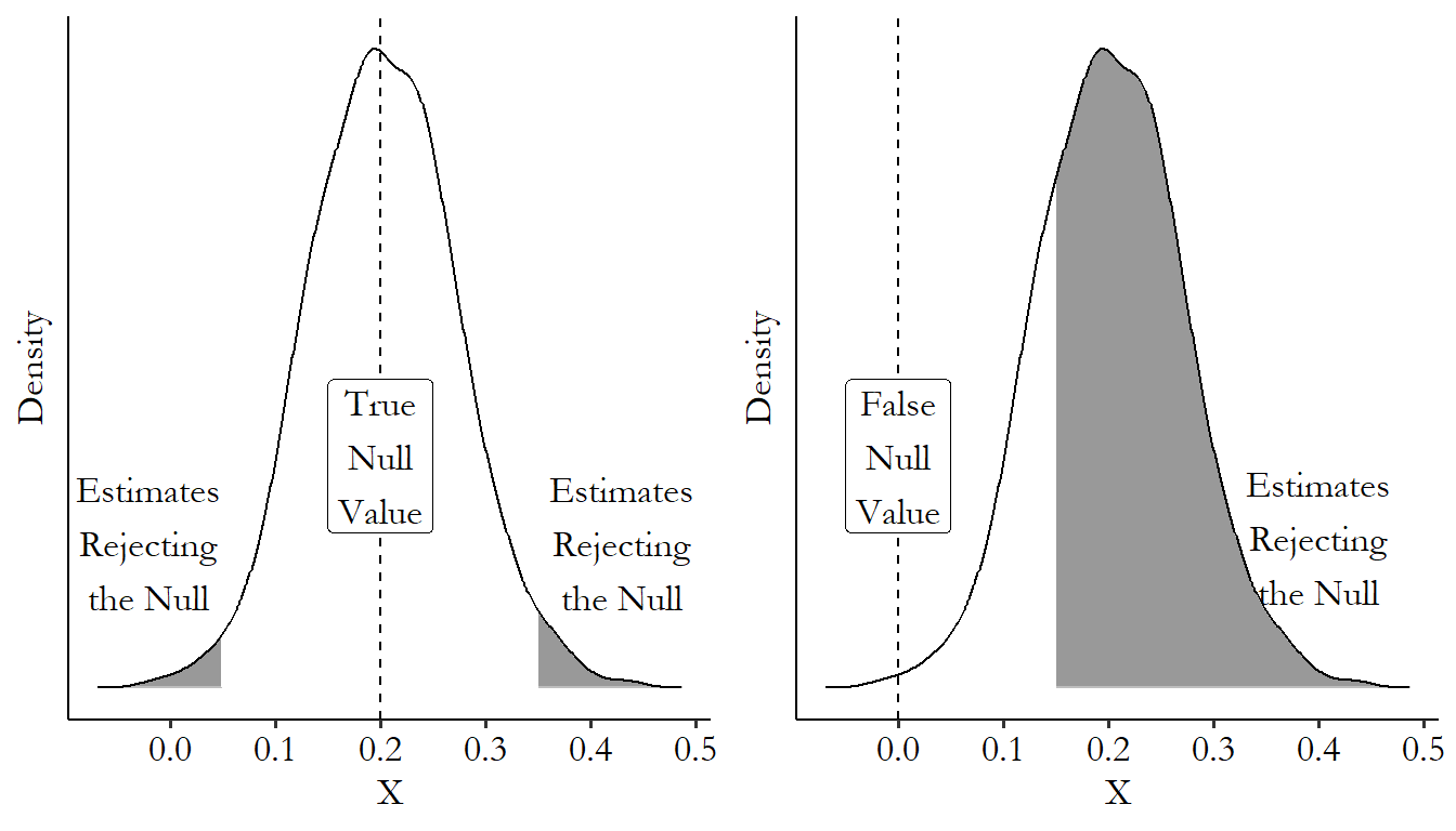
Figure 13.4: Testing 1,000 Randomly Generated Samples Against the True Null and a False Null
In practice, when applied to regression in most contexts, we’re talking about a normally-distributed regression coefficient and an \(\alpha = .05\) false positive rate (with a two-tailed test), testing against a null that the coefficient is 0. So if the probability of our estimate (or something even farther from 0) occurring is less than 5%, we call that “statistically significant” and say the relationship is nonzero.
The calculation of the probability comes from computing the percentiles of the normal distribution with a mean of 0 and a standard deviation of our estimated \(se(\hat{\beta}_1)\). If our estimate \(\hat{\beta}_1\) is below the 2.5th percentile or above the 97.5th, that’s statistically significant with \(\alpha = .05\).
We can also look at the exact percentile we get and evaluate that. If, for example, we find that our estimate of \(\hat{\beta}_1\) is at the 1.3rd percentile, then we can double that to 2.6, and say that we have a 2.6% probability of being that far away from the null or farther. This probability is called the “p-value.” The lower that p-value is, the lower the chance is of finding a result that far from the null or farther by sampling variation alone. If you look back at Figure 13.3, the entire shaded area is the p-value, since it’s the area as far away from the null as the actual estimate is, or farther. If the p-value is below \(\alpha\), that’s statistical significance.
p-value. The probability of getting an estimated result as far from the null (or farther), given the theoretical sampling distribution based on the chosen null-hypothesis value.
Using some known properties of the normal distribution, we can take a shortcut without having to go to the trouble of calculating percentiles. In this context, the t-statistic is the coefficient divided by its standard error \(\hat{\beta}_1/se(\hat{\beta}_1)\). When we scale the estimate by its standard error, that puts us on the “standard normal” theoretical distribution where the standard deviation is 1. Then, if that t-statistic is below -1.96 (the 2.5th percentile) or above 1.96 (the 97.5th percentile), that’s statistically significant at the 95% level, and a nonzero relationship.
Using that sort of interpretation is what lets us read regression tables, which we’ll get to in a second. But before we do, one aside on this whole concept of statistical significance. Rather, a plea.
Having taught plenty of students in statistical methods, and, further, talked with plenty of people who have received teaching in statistical methods, the single greatest difference between what students are taught and what students learn is about statistical significance. I think this is because significance is wily and tempting.209 If the Lord of the Rings were statistics, significance testing would be the One Ring. Not to mention all the people trying to throw it into a volcano. Of course if Lord of the Rings really were statistics, they wouldn’t have made those movies about it. Powerful, tempting, seemingly simple, but so easy to misuse, and so easy to let it take you over and make you do bad things. So please keep the following things in mind and repeat them as a mantra at every possible moment until they live within you:
- An estimate not being statistically significant doesn’t mean it’s wrong. It just means it’s not statistically significant.
- Never, ever, ever, ever, ever, ever, ever give in to the thought: “oh no, my results aren’t significant, I’d better change the analysis to get something significant.” Bad.210 Why? First off, maybe there truly just isn’t much of an effect. Insignificant doesn’t mean wrong! Also, changing the analysis to seek significance makes your future significance tests incorrect and meaningless - the tests all assume that you don’t do this. Your results become garbage, even if they look nice and you can fool people into thinking they’re good. I’m pretty sure professors always say to never do this, but students somehow remember the opposite.211 To be fair, sometimes researchers do this too. It’s called ``p-hacking,’’ where you keep changing your statistical analysis until you find some way to produce a statistically significant result. It’s bad. It’s a bad thing that is bad when it’s done because it’s bad to do and it makes the results bad. Bad.
- A lot of stuff goes into significance besides just “is the true relationship nonzero or not.” - sampling variation, of course, and also the sample size, the way you’re doing your analysis, your choice of \(\alpha\), and so on. A significance test isn’t the last word on a result.212 That said, speculating on whether an insignificant result would become significant with, say, a bigger sample size generally isn’t too useful.
- Statistical significance only provides information about whether a particular null value is unlikely. It doesn’t say anything about whether the effect you’ve found matters. In other words, “statistically significant” isn’t the same thing as “significant.”213 Even though researchers, myself included, will often just say “significant” as a shorthand for statistically significant. A result showing that your treatment improves IQ by .000000001 points is not a meaningful effect, whether it’s statistically significant or not.
Keep in mind, generally: the point of significance testing is to think about not just the estimates themselves but also the precision of those estimates. If you’ve got a really cool result but the standard errors are huge, there’s a good chance it’s a fluke that could be consistent with lots of true relationships. That’s the kind of thinking significance testing is meant to encourage. But there are other ways to keep precision in mind. You could just think about the standard errors themselves; ask if the estimate is precise regardless of whether it’s far from a given null value. You could ask what the range of reasonable null values is (construct a confidence interval) instead of focus on one in particular. You could go full Bayesian and do whatever the heck it is those crazy cats get up to. Significance testing is just one way of doing it, and it has its pros and cons like everything else.
13.1.4 Regression Tables and Model-Fit Statistics
We have a decent idea at this point of how to think about the line that an OLS estimation produces, as well as the statistical properties of its coefficients. But how can we interpret the model as a whole? How can we make sense of a whole estimated regression at once? For that we can turn to the most common way that regression results are presented: the regression table.
We’re going to run some regressions using data on restaurant and food inspections. We might be curious whether chain restaurants get better health inspections than restaurants with fewer (or only one) location.214 This data comes from Louis-Ashley Camus on Kaggle We’ll be using this data throughout this chapter. Some basic summary statistics for the data are in Table 13.1. We have data on the inspection score (with a maximum score of 100), the year the inspection was performed, and the number of locations that restaurant chain has.
Table 13.1: Summary Statistics for Restaurant Inspection Data
| Variable | N | Mean | Std. Dev. | Min | Pctl. 25 | Pctl. 75 | Max |
|---|---|---|---|---|---|---|---|
| Inspection Score | 27178 | 94 | 6.3 | 66 | 90 | 100 | 100 |
| Year of Inspection | 27178 | 2010 | 5.9 | 2000 | 2006 | 2016 | 2019 |
| Number of Locations | 27178 | 65 | 84 | 1 | 27 | 71 | 646 |
Now I’ll run two regressions. The first just regresses inspection score on the number of locations the chain has:
and the second adds year of inspection as a control:
I then show the estimated results for both in Table 13.2.
| Inspection Score | Inspection Score | |
|---|---|---|
| (Intercept) | 94.866*** | 225.333*** |
| (0.046) | (12.411) | |
| Number of Locations | −0.019*** | −0.019*** |
| (0.000) | (0.000) | |
| Year of Inspection | −0.065*** | |
| (0.006) | ||
| Num.Obs. | 27178 | 27178 |
| R2 | 0.065 | 0.068 |
| R2 Adj. | 0.065 | 0.068 |
| F | 1876.705 | 997.386 |
| RMSE | 6.05 | 6.04 |
| * p < 0.1, ** p < 0.05, *** p < 0.01 |
What can we see in Table 13.2? Each column represents a different regression. The first column of results shows the results from the Equation (13.2) regression, and the second column of results shows the results from the Equation (13.3) regression.
The first thing we notice is that each variable used to predict Inspection Score gets its own set of two rows. The “Intercept” also gets two rows - this is \(\hat{\beta}_0\), and on some tables is called the “Constant.” The first row shows the coefficient estimate. Our estimate \(\hat{\beta}_1\), the coefficient on Number of Locations, is \(\hat{\beta}_1 = -.0019\). It happens to be the same in both regressions - the addition of Year as a control didn’t change the estimate enough to notice. There are also some asterisks - I’ll get to those in a second.
Below the coefficient estimates, we have our measures of precision, in parentheses.215 Some regression tables put the precision measures to the right of the coefficient rather than below, so you’d have two columns for each regression. In particular, in this table these are the standard errors of the coefficients. \(se(\hat{\beta}_1)\) in this regression is \(.0004\) - seems pretty precise to me. There are a few different ways you can measure the precision of a coefficient estimate. Putting standard errors here is the most common, but sometimes you’ll see something like a confidence interval. In some fields, using a t-statistic (coefficient divided by the standard error) is more common than the standard error. Ideally a table will tell you which one they’re doing, but not always!216 If it doesn’t say, it’s usually a standard error, and if it’s a single number it’s almost always a standard error or a t-statistic. You can tell which of those two it is by looking at the significance stars - if precision values that are big relative to their coefficients give you significance, that’s probably a t-statistic. If small values relative to the coefficients give you significance, that’s probably a standard error.
Finally, we have those asterisks, called “significance stars.” These let you know at a glance whether the coefficient is statistically significantly different from a null-hypothesis value of 0. To be really precise, these aren’t exactly significance tests. Instead, they’re a representation of the p-value.217 Remember, the p-value is the probability of being as far away from the null hypothesis value (or farther) as our estimate actually is. If the p-value is below \(\alpha\), that’s statistical significance. The lower the p-value is, the more stars we get.
Which p-value cutoff each number of stars corresponds to changes from field to field but should be described in the table note as it is here. A standard in many of the social sciences, and what you’ll see in this book, is that * means that the p-value is below .1 (10%), ** means it’s below .05 (5%), and *** means it’s below .01 (1%).218 In many fields, and in most R commands by default, everything is shifted over one step. * is below .05, ** is below .01, and *** is below .001. There’s often another indicator in these cases like + for .1. So if we see *** as we do in this table for the coefficient on Number of Locations, that would mean that if we had decided that \(\alpha = .01\) (or higher), we would reject the null of \(\beta_1 = 0\). If we see ** then we’d find statistical significance at \(\alpha = .05\) or higher. Basically, it’s a measure of which \(\alpha\) values you’d find significance with for this coefficient.219 This is a bit backwards - we generally want to choose a \(\alpha\) value before we start. What’s the point of knowing significance tests at higher \(\alpha\) values? We already said that doesn’t count. And if our \(\alpha = .05\), then *** doesn’t really give us additional information - something is either significant or it’s not. There’s no such thing as “more significant.” Of course, I’m describing an idealized version of significance testing that people don’t actually do. These stars are a way of, at a glance, being able to tell which of the coefficients are statistically significantly different from 0, which all of these are.
Moving down the table, we have a bunch of things that aren’t coefficients or precision measures. Which of these exact statistics are present will vary from table to table,220 Some other common appearances here might be an information criterion or two (like AIC or BIC, the Akaike and Bayesian Information Criterion, respectively) or the sum of squares. I won’t be covering these here. but in general these are either descriptions of the analysis being run, or measures of the quality of the model. For the first, it’s common to see any additional details about estimation listed down here (such as any standard error adjustments), and just about every table will tell you the number of Observations (or sometimes “N”) included in estimating the regression.
For the second, there are a billion different ways to measure the quality of the model. Probably two of the most common are included here - \(R^2\) and Adjusted \(R^2\). These are measures of the share of the dependent variable’s variance that is predicted by the model. \(R^2\) in the first model is \(.065\), telling us that 6.5% of the variation in Inspection Score is predicted by the Number of Locations. If we were to predict Inspection Score with Number of Locations and then subtract out our prediction, we’d be left with a residual variable that has only \((100 - .065 = )\) 93.5% of the variance of the original. Adjusted \(R^2\) is the same idea, except that it makes an adjustment for the number of variables you’re using in the model, so it only counts the variance explained above and beyond what you’d get by just adding a random variable to the model.221 Yes, adding a random variable to the model does explain more of its variation. In fact, adding any variable to a model always makes the \(R^2\) go up by some small amount, even if the variable doesn’t make any sense.
Finally, we have the “F-statistic.” This is a statistic used to do a hypothesis test. Specifically, it uses a null that all the coefficents in the model (except the intercept/constant) are all zero at once, and tests how unlikely your results are given that null. It’s pretty rare that this will be insignificant for any halfway-decent model, and so I for one mostly ignore this statistic.
Missing from this particular table, but present in a number of standard regression-table output styles, is the residual standard error, sometimes also called the root mean squared error (RMSE). This is, simply, our estimate of the standard deviation of the error term based on what we see in the standard deviation of the residuals. We take our predicted Inspection Score values based on our OLS model and subtract them from the actual values to get a residual. Then, we calculate the standard deviation of that residual and make a slight adjustment for the “degrees of freedom” - the number of observations in the data minus the number of coefficients in the model. The bigger this number is, the bigger the average errors in prediction for the model are.
What can we do with all of these model-quality measures? Take a quick look, but in general don’t be too concerned about these. These are usually measures of how well your dependent variable is predicted by your OLS model. But if you’re reading this book, you’re probably not that concerned with prediction. You’re interested in identifying causal effects, and in estimating particular coefficients well, rather than predicting the dependent variable overall.
If your \(R^2\) or adjusted \(R^2\) values are low, or your residual standard error is high, what this tells you is that there’s a lot going on with your dependent variable other than what you’ve modeled. Is that a concern? Maybe. If you thought you wrote down a diagram that explained your dependent variable super well and covered all of the things that cause it, and you chose your model and which variables to control for based on that… and then you got a tiny \(R^2\) anyway, then your initial assumption that you really understood the data generating process of your dependent variable might be wrong. But if you don’t care about most of the causes of your dependent variable and are pretty sure you’ve included the variables in your model necessary to identify your treatment, then \(R^2\) is of little importance.
Similar to statistical significance, I see \(R^2\) values as another thing that students tend to fixate on. Gets their buns in a knot.222 I don’t know what this means. But while it can be a nice diagnostic, it’s definitely not something to fixate on. Certainly don’t design your model around maximizing \(R^2\) - build the right model for identifying the effect you want to identify and answer your research question, not the right model for predicting the dependent variable. Even if you are interested in prediction, \(R^2\) has plenty of flaws in use for building predictive models too, although that’s another book.
Knowing where all the pieces of a regression are on a regression table, how can we interpret the results? Let’s take a look at the regression table again in Table 13.3.
| Inspection Score | Inspection Score | |
|---|---|---|
| (Intercept) | 94.866*** | 225.333*** |
| (0.046) | (12.411) | |
| Number of Locations | −0.019*** | −0.019*** |
| (0.000) | (0.000) | |
| Year of Inspection | −0.065*** | |
| (0.006) | ||
| Num.Obs. | 27178 | 27178 |
| R2 | 0.065 | 0.068 |
| R2 Adj. | 0.065 | 0.068 |
| F | 1876.705 | 997.386 |
| RMSE | 6.05 | 6.04 |
| * p < 0.1, ** p < 0.05, *** p < 0.01 |
A key phrase to keep in mind when interpreting the results of an OLS regression is “a one-unit change in…” Regression coefficients are all about estimating a linear relationship between two variables, and reporting the results in terms of the slope, i.e., the relationship between a one-unit change in the predictor variable and the dependent variable.223 Sometimes regression results are presented as “standardized coefficients” for which this becomes “a one-standard-deviation change in…” But you can also just think of it as a “one-unit change” for variables scaled to have a standard deviation of 1.
If we want to get real precise about it, the interpretation of an OLS coefficient \(\beta_1\) on a variable \(X\) is “controlling for the other variables in the model, a one-unit change in \(X\) is linearly associated with a \(\beta_1\)-unit change in \(Y\).” If we want to get even more precise, we can say “If two observations have the same values of the other variables in the model, but one has a value of \(X\) that is one unit higher, the observation with the \(X\) one unit higher will on average have a \(Y\) that is \(\beta_1\) units higher.”
Let’s start with the first column of results, with only one variable, a \(-.019\) on Number of Locations. Let’s think briefly about our units here. Number of Locations is the number of locations in the restaurant chain, and the dependent variable, Inspection Score, is an inspector score on a scale that goes up to 100.
Since we have no other control variables in the model, that \(-.019\) means “a one-unit increase in the number of locations a chain restaurant has is linearly associated with a \(-.019\)-point decrease in inspector score, on a scale of 0-100.” Or, “comparing two restaurants, the one that’s a part of a chain with one more location than the other will on average have an inspection score \(-.019\) lower.”
Notice that however I’m wording it, I’m careful to avoid saying “a one-unit increase in number of locations decreases inspector score by \(-.019\).” This would be implying that I’ve estimated a causal effect. I should only use this language if, based on what we learned in the first part of the book, we think we’ve identified the causal effect of number of locations on inspector score.
How about that constant term 94.866? This is our prediction for the dependent variable when all the predictor variables are zero. Think about it - our conditional mean of the dependent variable is whatever the OLS model spits out when we plug the appropriate values in. If we plug in 0 for everything, it all drops out and all we have left is our constant. So for a restaurant with zero locations, we’d predict an inspector score of 94.866. Of course, it’s impossible to have a restaurant with zero locations, so this doesn’t mean much.224 If you have predictor variables where the relevant range of the data is far away from zero, the constant term can sometimes give strange values. This isn’t a problem - just don’t try to make predictions far outside the range of your data. In general we don’t need to worry ourselves too much about the constant term.
Let’s move to the second column. We’re introducing a control variable here, year of inspection. It doesn’t seem to change the coefficient on number of locations, but it does change the interpretation.
Now we need to incorporate the fact that our interpretation of each coefficient is based on the idea that we are “controlling for” the other variables in the model.225 i.e., closing the back doors that go through those variables. We can say this in a few ways.
We can say “controlling for year of inspection, a one-unit increase in the number of locations a chain restaurant has is linearly associated with a \(-.019\)-point decrease in inspector score, on a scale of 0-100.” Instead of “controlling for” we could instead say “adjusting for” or “adjusting linearly for” or even “conditioning on.”226 Remember the “conditional mean” stuff from Chapter 4? That’s the kind of “conditioning” I mean.
We can say “comparing two inspections in the same year, the one for a restaurant that’s a part of a chain with one more location than the other will on average have an inspection score \(-.019\) lower.” After all, that’s the idea of controlling for variables. We want to compare like-with-like and close back doors, and so we’re trying to remove the part of the Number of Locations/Inspector Score relationship that is driven by Year of Inspection. The idea is that by including a control for Year, we are removing the part explained by Year, and can proceed as though the remaining estimates are comparing two inspections that effectively have the same year. There’s no variation in year left - we have held year constant.227 Or at least we’ve held its linear predictions constant. If Year of Inspection relates to Inspector Score or Number of Locations in ways that are best described by curvy lines, then including Year of Inspection as a linear predictor in the regression equation won’t fully control for it. For this reason you will also often hear the interpretation “holding year of inspection constant, a one-unit increase in the number of locations is associated with a \(-.019\) decrease in inspector score.”
This is a simple guide to interpreting a regression, and one that’s focused pretty heavily on semantics. But training yourself to explain regression in these terms will truly help you interpret them better. The same intuition will carry over when you start doing regression in more complex settings, as we’ll discuss throughout the chapter.
13.1.5 Subscripts in Regression Equations
I’ve left out one common feature of expressing a regression. When writing out the equation for a regression, people will commonly use subscripts on their variables (i.e., \(X_{little text down here}\)). We already have subscripts on our coefficients (the 1 in \(\beta_1\), etc.), but they show up on the variables themselves, too. I’ve chosen mostly to omit these in this book,228 I’ve got nothing against them! But I think at the level we’re working they’re more distracting than helpful. but it’s important to be familiar with the concept when you’re reading papers or writing your own.
A regression might be expressed as
The \(i\) here tells us what index the data varies across. In other words, a single observation is a what exactly? Here we have \(i\), which generally means “individual,” i.e., an individual person or firm or country, depending on context. In this regression, \(Y\) and \(X\) differ across individuals.
Alternately, we might see
The \(t\) here would be shorthand for time period. This is describing a regression where each observation is a different time period. The \(X_{t-1}\) tells us that we are relating \(Y\) from a given period \(t\) to the \(X\) from the period before \((t-1)\).
The subscripts do their best work when there are multiple axes that things could vary along. Consider this example:
This is describing a regression in which \(Y\) and \(X\) vary across a set of individuals \(i\) and across time \(t\) (a panel data set). There is a different intercept for each time period \(\beta_t\), and also a different intercept for each value of \(g\) (and what’s \(g\)? We’d have to look for where the researcher is describing their regression, but it might mean some \(g\)rouping that the individuals \(i\) are sorted into). We also see a control variable \(W_i\). The \(i\) subscript here (and lack of a time subscript \(t\)) tells us that \(W\) only varies across individual and doesn’t change over time. Perhaps \(W\) is something like birthplace that is different for individuals but does not vary over time.
13.1.6 Turning a Causal Diagram into a Regression
Okay, so we’ve covered the basics of how regression works. And we spent the first half of this whole book talking about how to identify causal effects using causal diagrams.
It’s tempting to think that we automatically know how to link the two, but I’ve found that students often have difficulty making this jump. It’s not a super difficult jump, mind you, but it’s not one we can take for granted.
The chart in Figure 13.5 may help. On the diagram, we’re thinking about what to do with a variable \(A\). Is it the outcome variable, or is some other variable \(Y\) the outcome? Is it the treatment, or is some other variable \(X\) the treatment? If it’s neither, where does it go on the diagram and also in a regression, if anywhere at all?
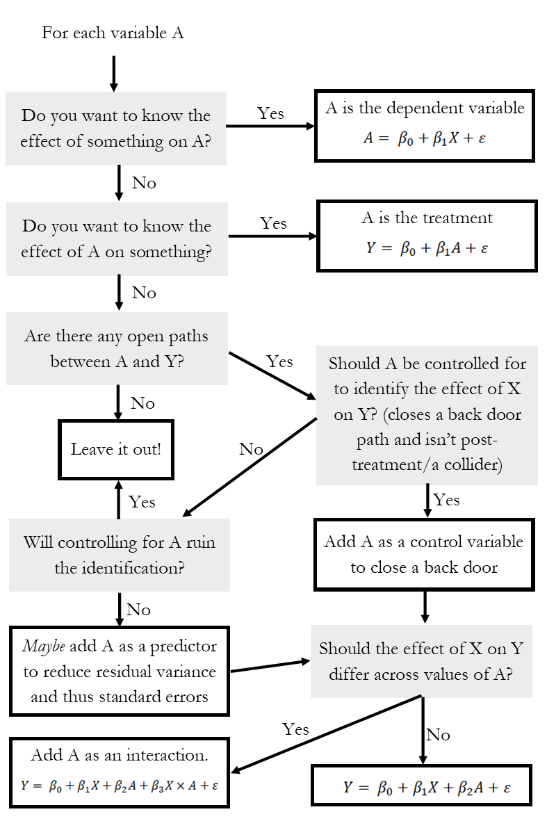
Figure 13.5: Chart for Constructing a Regression Equation
As shown in Figure 13.5, each variable may play one of several roles in a regression. It could be our outcome variable - we know all about those. Outcome variables become the dependent variables in regression, the \(Y=\) part of \(Y = \beta_0 +\beta_1X\). We know all about treatment variables from our discussion of causal diagrams, too. Those become the \(\beta_1X\) part.
How about the rest? Our causal diagram tells us all about variables that need to be adjusted for in order to close back doors (and also those that shouldn’t be controlled for to avoid closing front doors or opening back doors by controlling for colliders). Anything that should be included as a control should be, well, included as a control. That’s the \(+\beta_2A\) part of \(Y = \beta_0+\beta_1X+\beta_2A\), where \(X\) is the treatment and \(Y\) is the outcome.
There are two things we haven’t come to yet that show up in regression but not so much in causal diagrams. First, what if a variable \(A\) doesn’t need to be controlled for, but also controlling for it won’t break the identification? In that case we can include it as a control, and maybe we want to - as long as \(A\) is related to \(Y\), then adding it will explain more of the variation in \(Y\), reducing variance in the error term. And since the standard errors of the regression coefficients like \(\hat{\beta}_1\) rely on the variance of the error term, the standard errors will shrink.
Finally, what about that part of the graph where it asks about whether the effect of treatment will differ across values of \(A\)? That’s where interaction terms come in. We’ll talk about those later in the chapter.
13.1.7 Coding Up a Regression
Before we move on, we should probably actually do a regression. Seems like a good idea.
The following code chunks will replicate Tables 13.2 and 13.3 in R, Stata, and Python. They will load in the restaurant inspection data, calculate the number of locations, regress inspection score on the number of locations, do another regression that also includes year as a control, and then output a regression table to file.
Note that while the code for performing a regression is fairly standard in each language, the process for producing a regression table generally depends on downloadable packages. There are plenty of options for these packages. I’ll be using the modelsummary R package (install.packages('modelsummary')), estout for Stata (ssc install estout), and stargazer for Python when there’s more than one regression to display (pip install stargazer). But some good alternatives include export_summs from the jtools package, or outreg2, regsave, or the Stata 17 exclusive collect in Stata.229 I recognize that estout is probably the better package for Stata regression tables and that’s why I use it here. I’ve heard good things about regsave, but I personally will use outreg2 until the day that I die. You shall pry its arcane syntax, and the head-scratching fact that it is less up-to-date than outreg, from my cold dead fingers.
R Code
library(tidyverse); library(modelsummary)
res <- causaldata::restaurant_inspections

res <- res %>%
    # Create NumberofLocations
    group_by(business_name) %>%
    mutate(NumberofLocations = n())

# Perform the first, one-predictor regression
# use the lm() function, with ~ telling us what
# the dependent variable varies over
m1 <- lm(inspection_score ~ NumberofLocations, data = res)

# Now add year as a control
# Just use + to add more terms to the regression
m2 <- lm(inspection_score ~ NumberofLocations + Year, data = res)

# Give msummary a list() of the models we want in our table
# and save to the file "regression_table.html"
# (see help(msummary) for other options)
msummary(list(m1, m2),
    stars=TRUE,
    output= 'regression_table.html')
# Default significance stars are +/*/**/*** .1/.05/.01/.001. Social science
# standard */**/*** .1/.05/.01 can be restored with
msummary(list(m1, m2),
    stars=c('*' = .1, '**' = .05, '***' = .01),
    output= 'regression_table.html')
Stata Code
* ssc install causaldata if you haven't yet!
causaldata restaurant_inspections.dta, use clear download

* Create NumberofLocations
by business_name, sort: g NumberofLocations = _N

* Perform the first, one-predictor regression
regress inspection_score NumberofLocations
* Store our results for estout
estimates store m1

* Now add year as a control
regress inspection_score NumberofLocations year
estimates store m2

* use esttab to create a regression table
* note esttab defaults to t-statistics, so we use
* the se option to put standard errors instead
* we'll save the result as regression_table.html
* (see help esttab for other options)
esttab m1 m2 using regression_table.html, se replace
Python Code
import pandas as pd
import statsmodels.formula.api as smf
from stargazer.stargazer import Stargazer
from causaldata import restaurant_inspections

res = restaurant_inspections.load_pandas().data

# Perform the first, one-predictor regression
# use the sm.ols() function, with ~ telling us what
# the dependent variable varies over
m1 = smf.ols(formula = 'inspection_score ~ NumberofLocations',
data = res).fit()

# Now add year as a control
# Just use + to add more terms to the regression
m2 = smf.ols(formula = 'inspection_score ~ NumberofLocations + Year',
data = res).fit()

# Open a file to write to
f = open('regression_table.html', 'w')
# Give Stargazer a list of the models we want
# in our table and save to file
regtable = Stargazer([m1, m2])
f.write(regtable.render_html())
f.close()
13.2 Getting Fancier with Regression
Regression is a tool - a very flexible tool. And we’ve only really learned one way to use it! This section isn’t even going to change how we use it; it’s just going to change the variables that go into it. This in itself will open up a whole new world.
So far, we’ve talked about regression of the format \(Y = \beta_0 + \beta_1X + \beta_2Z+ \varepsilon\). We’re still working with that. But we’ve also always been working with continuous variables included in the regression as their normal selves. Is there something else?
First, we might not have continuous variables. Instead, we might have discrete variables, which most often pop up as binary variables - true or false, rather than a particular number. How can we interpret \(\beta_2\) if \(Z\) is “this person has blonde hair”? Or, how would we control for “hair color” if that’s not a variable we’ve measured continuously, and we instead have categories like “black,” “brown,” “blonde,” and “red”?
Second, we might not use variables as they are but first transform them. We talked way back in Chapter 4 that some relationships might not be well-described by straight lines. Sometimes we want curvy lines. How can we do that, exactly?
Third, the relationships themselves might be affected by other variables. For example, back in Chapter 4 we talked about a study by Emily Oster that asked “is the relationship between taking vitamin E and health outcomes stronger during the period when vitamin E was recommended by doctors than during the periods when it wasn’t?” We can model the relationship between taking vitamin E and health outcomes with \(Outcomes = \beta_0 + \beta_1VitaminE+\varepsilon\). But how can we model how that relationship changes over time? We need an interaction.
So those three things - all of which have to do with the kinds of variables we use as predictors in our OLS model - will be where we start. Once we’ve covered that, we’ll move on to how we deal with standard errors, and when our dependent variable isn’t continuous either.
13.2.1 Handling Discrete Variables
Binary variables are absolutely everywhere in social science. Did you get the treatment or not? Are you left-handed or right-handed? Are you a man or a woman?230 Some people point out this should not be treated as a binary variable. I hope those people know how hard they’re making regression analysis. Think of the researchers. Are you Catholic or not? Are you married or not?
Binary variables are especially important for causal analysis, since a lot of the causes we tend to be interested in are binary in nature. Did you get the treatment or not?
Any time we have something that you are or are not, which happens any time we have some sort of qualitative description, we are dealing with a binary variable. These can be included in regression models just as normal. So we can still be working with \(Y = \beta_0 + \beta_1X + \beta_2Z+ \varepsilon\), but now maybe \(X\) or \(Z\) (or both) can only take two values: 0 (“are not”/false) or 1 (“are”/true).231 Sometimes you’ll see people use -1 and 1, or 1 and 2, instead of 0 and 1. This is usually just confusing though, and pretty rare in the social sciences. If the binary variable is a control variable, we can think of it as we normally do - we’re just shutting off back doors that go through the variable. But what if we are interested in the effect of that binary variable? How can we interpret the binary variable’s coefficient?
Simply put, it’s the difference in the dependent variable between the trues and the falses.232 Why is this? OLS is trying to fit a line that minimizes squared residuals. But there are only two values the data can take on the \(x\)-axis: 0 and 1. Because of that, the OLS line can only produce two real predictions: one when it’s 0 on the \(x\)-axis, and one when it’s 1. The best prediction you can make in each case, which minimizes the squared residuals is just the mean of the outcome conditional on the binary variable being 0 or 1. Then, the slope of the line is just how much the prediction increases when the \(x\)-axis variable increases by 1 (i.e., goes from 0 to 1). So for example, if we ran the regression \(Sales = \beta_0 + \beta_1Winter + \varepsilon\), where \(Winter\) is a binary variable that’s 1 whenever it’s Winter and 0 when it’s not, then \(\beta_1\) would be how much higher sales are on average in Winter than in Not Winter.233 And if sales are lower on average in Winter, \(\beta_1\) would be negative.
When we estimate the model, if we got \(\hat{\beta}_1 = -5\), then we’d say that, on average, sales are 5 lower in Winter than they are in Not Winter. Take a look at the simulated data in Table 13.4. Notice that the coefficient on Winter (-5) is just the difference between the mean for Not Winter (15) and the mean for winter (10). Also notice that the coefficient on the intercept (15) is the expected mean when all the variables are zero - when Winter is 0, we’re in Not Winter, and average sales in Not Winter are 15.
Table 13.4: Average Sales by Season, or Regression of Sales on Winter
| Mean | OLS Estimates | |
|---|---|---|
| Winter | 10.000 | -5.000 |
| (1.103) | ||
| Not Winter | 15.000 | (Ref.) |
| (Intercept) | 15.000 | |
| (3.413) |
Note: Standard errors are in parentheses. No significance stars are shown.
One important thing to note is that we only include one side of the yes/no question. The model is \(Sales = \beta_0 + \beta_1Winter + \varepsilon\), not \(Sales = \beta_0 + \beta_1Winter + \beta_2NotWinter + \varepsilon\). Why is this? First off, imagine trying to interpret that. We want \(\beta_1\) to compare Winter to Not Winter, but \(\beta_2\) compares Not Winter to Winter. So… what’s the difference between them? Interpretation would be pretty confusing. Second, this is to satisfy another OLS assumption we have to make, that there is no perfect multicollinearity. That is, you can’t make a perfect linear prediction of any of the variables in the model with any of the other variables. Here, \(Winter + NotWinter = 1\). We don’t have a 1 in our model, though, so no problem, right? Wrong! There is an all-1s variable lurking in our model at all times—it’s being multiplied by the constant!
Why can’t we have that linear combination? Because OLS wouldn’t be able to figure out how to estimate the parameters. Imagine the average sales in Winter are 10, and in Not Winter it’s 15. If your regression is \(Sales = \beta_0 + \beta_1Winter + \beta_2NotWinter + \varepsilon\), you could generate those exact same predictions with \(\beta_0 = 15, \beta_1 = -5, \beta_2 = 0\). Or with \(\beta_0 = 10, \beta_1 = 0, \beta_2 = 5\). Or with \(\beta_0 = 3, \beta_1 = 7, \beta_2 = 12\). Or any infinite number of other ways! And while they’d all work, OLS has no way of picking one estimate out of those many, many options. It can’t give you a best estimate any more. We need to limit its options by dropping NotWinter, in effect forcing it to choose the \(\beta_0 = 15, \beta_1 = -5, \beta_2 = 0\) version.
We can expand our intuition about binary variables just a bit and give ourselves the ability to include categorical variables in our model. Binary variables are just yes/no. But categorical variables can take any number of categories. These include variables like “what country do you live in?” or “what decade were you born in?” You can’t answer these questions with yes and no, but they are discrete and mutually exclusive categories.234 Sometimes these categories might allow some overlap - some people do live in multiple countries, for example. But hopefully we can avoid these situations, or there are few enough of them we can just ignore them, as they make things much more difficult.
We can handle categorical variables by just giving each of the categories its own binary variable. So instead of one variable for “which country do you live in?” it’s one variable for “do you live in France?”, another for “do you live in Gambia?”, another for “do you live in New Zealand?” and so on. \(Income = \beta_0 + \beta_1France + \beta_2Gambia+ \beta_3NewZealand + ...\) If we’re including the categorical variable as a control, by including these binary variables for each category we can say that we’ve closed the back doors that go through, in this example, which country you live in.
And what if we want to interpret the coefficient on one of these binary categories? This is just a hair trickier than with a binary variable. Just like we couldn’t include both sides of the binary variable in the model (we had to put just Winter in the model, not Winter and NotWinter), we also can’t include every single category in the model. We need to drop one of them. The one we drop then becomes the “reference category.” All the coefficients are relative to that category.
Before, with binary variables, the coefficient gave the difference between “yes” and “no.” Now, with a categorical variable and a reference category, it’s the difference between “this category” and “the reference category.”
For example, if we drop France from our regression,235 This does not mean we’re dropping all the observations from France. It just means we’re removing the \(France\) binary variable from our regression. France becomes the reference category. If we then estimate \(Income = \beta_0 + \beta_1Gambia+ \beta_2NewZealand + ...\) and get \(\hat{\beta}_1 = .5\) and \(\hat{\beta}_2 = 3\), then that means average income in Gambia is .5 higher than average income in France and average income in New Zealand is 3 higher than average income in France. Both of the interpretations only take things relative to the reference category, not each other.
We can see this in the simulated data in Table 13.5, which includes data only for France, Gambia, and New Zealand. Notice that average income for Gambia (30.5) is \(.5\) higher than the average income for France (30), and the coefficient on Gambia when France is the reference category is \(.5\). Similarly, the average income for New Zealand (33) is 3 higher than France, and the coefficient is 3. The intercept is the average income when all the predictors are 0 - so it’s not Gambia, and it’s not New Zealand, meaning it must be France. The average income in France is 30, so the intercept is 30.
Table 13.5: Average Income by Country among France, Gambia, and New Zealand, or Regression of Income on Country
| Mean | OLS Estimates | |
|---|---|---|
| France | 30.000 | (Ref.) |
| Gambia | 30.500 | .500 |
| (.103) | ||
| New Zealand | 33.000 | 3.000 |
| (1.321) | ||
| (Intercept) | 30.000 | |
| (5.412) |
Note: Standard errors are in parentheses. No significance stars are shown.
This reference category stuff means that the coefficients on the categories (and their significance) have relatively little meaning on their own. They only have meaning relative to each other. The coefficients change completely if you change the reference category. If we made New Zealand the reference category instead, the coefficient on Gambia would change from .5 to -2.5.236 Can you spot why?
If you want to know whether a categorical variable has a significant effect as a whole, you don’t look at the individual coefficients. Instead, you look at all the category coefficients. This takes the form of a “joint F test,” where you compare the predictive power of the model against a version where the categorical variable has been removed as a predictor.
In R, the linearHypothesis command in the car package can perform the joint F test. You give it the full list of names of coefficients for the categories (which you can make yourself using paste and unique with a little effort, or the matchCoefs() function). Slightly easier to use is wald() in the fixest package, which lets you easily pattern-match variable names, although this also requires the use of fixest’s feols() regression function instead of lm(). In Stata, testparm i.cat will do a joint significance test of all the categories of the cat variable. In Python, if you use smf.OLS().fit() to create a regression results object, let’s say it’s called m1, then you can do a joint F test with m1.f_test(). You’ll need to read the documentation to see how to create a matrix or string indicating the factor variables to be tested.
13.2.2 Polynomials
Sometimes, a straight line isn’t enough. OLS assumes that the relationship between the dependent variable and each of the predictor variables can be described as a straight line (linear). If that’s not true, OLS will do a poor job. For example, look at Figure 13.6. The true relationship clearly follows the curvy line drawn on the right. If we try to estimate this relationship using a straight line, we get something that doesn’t fit very well, shown by the line on the left.
Figure 13.6: Math Scores and Intelligence: OLS and the True Model
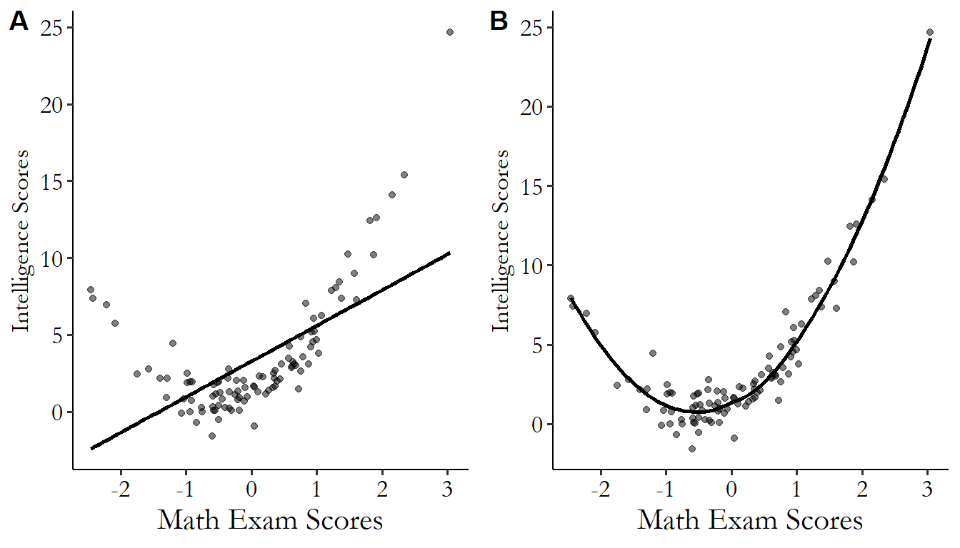
We can still use OLS for these kinds of relationships though. We just need to be careful to model that curviness right in our regression equation.
There are two main ways we can do this: we can either add polynomial terms, or we can transform the data.
A polynomial is when you have the same variable in an equation as itself, as well as powers of itself. So for example, \(\beta_1X + \beta_2X^2 + \beta_3X^3\) would be a “third-order polynomial” since it contains \(X\) to the first power (\(X\)), the second power (\(X^2\)), and the third power (\(X^3\)).237 These are also referred to as the linear, squared, and cubic terms, with quartic for the fourth power. \(^,\)238 Notice that this contains all the terms up to the third power. You pretty much never want to omit any, as in \(\beta_1X^2 + \beta_2X^3\) which has the second- and third-order terms but not the first.
By adding these polynomial terms, it’s possible to fit lines that aren’t straight. In fact, add enough terms and you can mimic just about any shape.239 Any functional relationship, that is - it still needs to make sense that we’re trying to get a single conditional mean of \(Y\) for each value of \(X\). This can be seen in Figure 13.7. Looking at the data points directly, this is clearly a nonlinear relationship. On top of the data points we have the best-fit line from a linear model (\(Y = \beta_0 + \beta_1X\)), which gives the straight line, a second-order polynomial model, which gives the curvy dashed line (\(Y = \beta_0 + \beta_1X + \beta_2X^2\)), and a third-order polynomial, which gives the curvy solid line (\(Y = \beta_0 + \beta_1X + \beta_2X^2 + \beta_3X^3\)).
Figure 13.7: Regression Using a Linear, Square, and Cubic Model
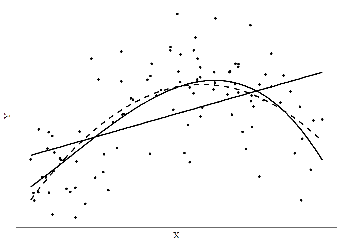
The curvy lines clearly do a better job fitting the relationship, and all we had to do was add those polynomial terms!
That’s the reason to add polynomial terms then. Add polynomial terms and you can better fit a line to a non-straight relationship. But this leaves us with two pressing questions: (1) how can we interpret the regression model once we have polynomial terms, and (2) why not just add a bunch of polynomial terms all the time?
How can we interpret a model with polynomials? For this one, we’re going to need a little calculus, I’m afraid. Let’s take our cubic model from before:
Our typical interpretation of a regression coefficient estimate like \(\hat{\beta}_1\) would be “holding everything else constant, a one-unit increase in \(X\) is associated with a \(\hat{\beta}_1\)-unit increase in \(Y\).” However, that’s a problem! We can’t “hold everything else constant” because there’s no way to change \(X\) without also changing \(X^2\) and \(X^3\). So an interpretation of the effect of \(X\) must take into account the coefficients on each of its polynomial terms. When a regression model includes a polynomial for \(X\), the individual coefficients on the \(X\) terms mean very little on their own, and must be interpreted together.
How can we interpret them together? Let’s try to get back our interpretation of “holding everything else constant, a one-unit increase in \(X\) is associated with a (???)-unit increase in \(Y\).” What is (???)? Well, what tool can we always reach for to figure out how one variable changes with another? The derivative! If we take the derivative of \(Y\) with respect to \(X\), that will tell us how a one-unit change in \(X\) is related to \(Y\).240 This works in a linear model too, of course. In \(Y = \beta_0 + \beta_1X\), the derivative of \(Y\) with respect to \(X\) is just \(\beta_1\). And thus we have our standard interpretation of \(\beta_1\) from a linear model.
A one-unit change in \(X\) is associated with a \((\beta_1 + 2\beta_2X+ 3\beta_3X^2)\)-unit change in \(Y\).241 Even if you don’t know calculus, if all you’ve got is a polynomial, this is a derivative that’s easy enough to do yourself. Just take each term, multiply it by its exponent, and then subtract one from the exponent (keeping in mind that \(X = X^1\), and when you subtract one from that exponent you get \(X^0 = 1\)). So \(\beta_3X^3\) gets multiplied by its exponent of 3 to get \(3\beta_3X^3\), and then we subtract one from the exponent to get \(3\beta_3X^2\). Repeat with each term. Notice that the relationship varies with different values of \(X\). If \(X = 1\), then the effect is \(\beta_1+ 2\beta_2+ 3\beta_3\). But if \(X = 2\), then it’s \(\beta_1 + 4\beta_2 + 12\beta_3\). The effect of \(X\) on \(Y\) depends on the value of \(X\) we already have. This is what we’d expect. Look back at Figure 13.7 - as \(X\) increases, at first \(Y\) increases as well, but then \(Y\) stops increasing and starts declining. The effect of a one-unit change in \(X\) should vary as we move along the \(X\)-axis.
Let’s use a more concrete example. Let’s go back to our regression from Table 13.2 but add a squared term, which we can see in Table 13.6.
| Inspection Score | |
|---|---|
| Constant | 97.5179*** |
| (0.0588) | |
| Number of Locations | −0.0802*** |
| (0.0010) | |
| Number of Locations Squared | 0.0001*** |
| (0.0000) | |
| Num.Obs. | 27178 |
| R2 | 0.194 |
| R2 Adj. | 0.194 |
| F | 3279.008 |
| RMSE | 5.62 |
| * p < 0.1, ** p < 0.05, *** p < 0.01 |
Here we see a coefficient of \(-.0802\) on the linear term, and \(.0001\) on the squared term. This means that a one-location increase in the number of locations associated with a restaurant chain is associated with a \(\beta_1 + 2\beta_2NumberofLocations\), or \(-.0802 + .0002NumberofLocations\), change in the health inspection score. So for a chain with only one location, adding a second one would be associated with a \(-.0802 + .0002(1) = -.0800\) reduction in the health score. But for a chain with 1000 locations, adding its 1001st would be associated with a \(-.0802 + .0002(1000) = .1198\) increase in its health score. There is no single effect; it depends on what part of the \(X\)-axis we’re on. Leaving out the squared term would ignore that.
Polynomials seem pretty handy! So why not just add a whole bunch of them all the time? And while we’re at it, why stop at just square terms and cubics? Why not add four-, five-, six-, or seven-order polynomials to all our models?
There are a few good reasons. For one, the model does get a little harder to interpret. Of course, if it’s the right model we’d still want that anyway.
For another, often the higher-order polynomial terms don’t really do anything. Take Figure 13.7 for example. The line fits from the second-order polynomial and the third-order polynomial models are almost exactly the same.242 And I can tell you, since I generated this data myself, that the true underlying model actually does have a cubic term. Despite this, the cubic term in the regression adds little to nothing. So in many cases, by adding more and more polynomial terms, you make your model more complex without actually improving its fit.
There is also the issue that adding polynomial terms puts strain on the data and can lead to “overfitting,” where a too-flexible model winds up bending in strange shapes to try to fit noise in the data, producing a worse model. Imagine, for example, fitting a 100-order polynomial on a data set with 100 observations in it. We’d predict every point perfectly, but clearly that line isn’t really going to tell us much of anything.
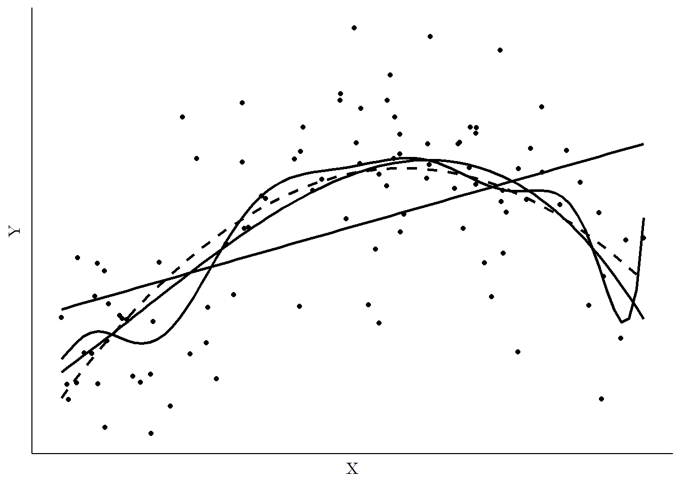
Adding more polynomial terms can, in general, make the model very sensitive to little changes in the data and can make its predictions kind of strange near the edges of the observed data. Take Figure 13.8, for example, which starts with Figure 13.7 and adds a regression fit using a ten-degree polynomial. The shape doesn’t seem to follow the data all that much better than even the two-order polynomial. And we get strange up-and-down motion that seems to chase individual observations rather than the overall relationship. The worst offender is over on the far right, where at the last moment the line springs way up to try to fit the single point on the far right of the data. Those additional degrees in the polynomial aren’t just unnecessary, they’re actively making the model worse.
Figure 13.8: Regression Using a Linear, Square, Cubic, and Ten-degree Polynomial Model
So we don’t want “too many” polynomial terms. But how much is just right? Well, ideally, you want to have the number of polynomial terms necessary to model the actual true underlying shape of the relationship. But we don’t actually know what that is, so that doesn’t help much.
A good way to approach the question of how many polynomial terms to include (or whether to include them at all) is graphically. This works best when you don’t have too many observations. Just draw yourself a scatterplot and see what the shape of the data looks like. Then, add your regression line and see whether it seems to explain the shape you see. If it doesn’t, try adding another polynomial term until it does.
You can also graphically analyze the residuals. Try a regression model, calculate the residuals, and then plot those on the \(y\)-axis against your \(x\)-axis variable. If you have enough polynomial terms, there shouldn’t be any sort of obvious relationship between \(X\) and the residuals. This can be seen in Figure 13.9. The same data from Figure 13.8 is estimated using a linear OLS and a second-order polynomial OLS, and the residuals from those regressions are plotted against \(X\). After the linear regression, there’s still a clear shape to the relationship between the residuals and \(X\) on the left. Not enough curviness to our line. But on the right, after our second-order polynomial, it’s just a bunch of noise around 0. That’s enough, we can stop!
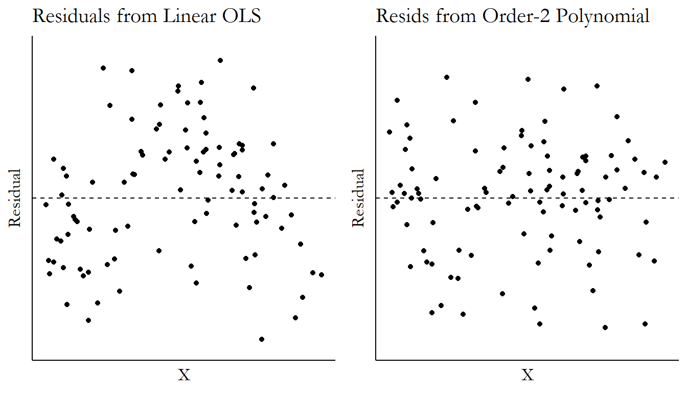
Figure 13.9: Residuals from Linear OLS and Second-Order Polynomial OLS
Besides all that, just as a good rule of thumb, you almost never want to go beyond cubic unless you have a really good reason. At that point you have to start worrying that the statistical issues with too many terms are going to be a problem. The cure of polynomials may be worse than the disease of nonlinearity.
There are also more automatic approaches to selecting the number of polynomials. You don’t have to look far to find people recommending that you try different amounts of polynomials, and then omit higher-order terms that are insignificant. In other words, try a quartic, and if the \(X^4\) coefficient is insignificant, drop it. Then try the cubic, and if the \(X^3\) term is insignificant… and so on. I don’t recommend this approach, as you are at this point making decisions about your model based on a statistical significance test, and that’s not what statistical significance tests are meant to do.243 Remember, “insignificant” doesn’t actually mean “this coefficient is zero.” It means “we don’t have evidence to show that it’s not zero.” Omitting it from the model forces it to be zero, which may not be right.
A somewhat better approach is to use a principled model-selection algorithm like a Least Absolute Shrinkage and Selection Operator (LASSO). Information on the specifics of LASSO will have to wait until the “Penalized Regression” section later in the chapter. For now, you can just think of it as a variant of OLS that tries to not just minimize the sum of squared errors, but it tries to do so while reducing the coefficients in the model. Like dropping polynomial terms because they’re insignificant, it takes the approach that additional polynomial terms that don’t improve prediction much can be dropped. However, it does so in a way that is actually designed for the purpose of figuring out whether an additional term is “worth it,” rather than using significance testing, which only by happenstance sort of tries for a similar goal.
13.2.3 Variable Transformations
Polynomial terms are not the only way to fit a nonlinear shape. In many cases it makes more sense to transform the variable itself directly.
Generally this means running a variable through a function before you use it. So for example, instead of running the regression
you might instead run
where \(\ln()\) is the base-\(e\) logarithm, or the “natural log.”244 What makes it so “natural”? Because whenever you have compounded growth (i.e., the interest you earn then starts earning its own interest, or the animal population reproduces, and then those babies grow up and reproduce as well), the number \(e\) will always be lurking around in your calculation somewhere, just like \(\pi\) will always be lurking around if you’re doing calculations about circles and curves.
Why might we do this? There are two main reasons we might want to transform a variable before using it, some of which we already covered in Chapter 3.245 “Wanting your variable to be normally distributed” is not a good reason to transform your variable. It’s a common myth that the variables you use in a regression need to be normally distributed. Regression standard error calculations care whether your error term is normally distributed (and even that isn’t super duper important as long as the error is somewhat well behaved), but for the variables themselves it does not matter.
The first reason might be to give the variable statistical properties that play more nicely with regression. For example, you may want to reduce skew. A variable is “right skewed” if there are a whole lot of observations with low values and just a few observations with really high values.246 Left skew would mean a whole lot of high values with just a few really low ones. This is less common than right skew in most social science research, though. Income is a good example of a skewed variable. Most people are somewhere near the median income, but a few super-high earners like CEOs and movie stars earn way way way more than the median.247 For more on skewed variables, refer back to Chapter 3.
Skewed data are likely to produce outlier observations. An outlier is an observation that has values that are very different from the other observations. For example, if you have a hundred people who all earn roughly $40,000 per year, and one person who earns a million, that person is an outlier.248 Outliers can come from non-skewed data, too.
There’s nothing inherently wrong with outlier observations. Sometimes people take big outliers as indications that the data has not been recorded properly and that million-dollar-salary is more likely a hundred-thousand with a typo, but often the data is fine, it’s just an outlier. However, even though the data may be accurate, the presence of outliers can make regression models statistically weak. Because the observations are way out there, they tend to produce big errors, and so just a few observations can have the effect of really tugging on the regression line and having way too much influence.
Outlier. An outlier is an observation with a value that is much bigger or smaller than the other observations.
Using a transformation that “scrunches down” the big observations to be closer to the others can reduce this skew, and make the regression model behave a bit better. This can be seen in Figure 13.10. On the left, we have raw data, with a single big outlier way to the top-right of the rest of the data. I’ve estimated OLS twice on this data, once leaving out the outlier and once including it. The estimated OLS slope changes wildly!
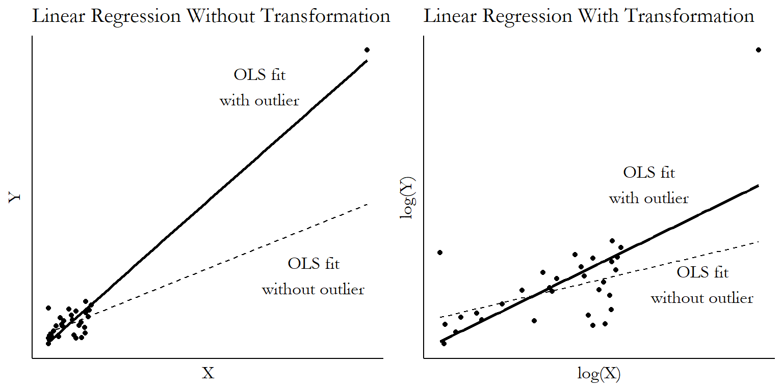
Figure 13.10: OLS Fit with and without an Outlier, with and without Log Transformations
On the right, I’ve taken the logarithm of both \(X\) and \(Y\). You can immediately see that the outlier comes in closer to the rest of the data (this shows up on the graph as the other data spreading out, since we can zoom in more closely on it without losing the outlier). The distance between observations is shrunk at the high end. Also, including or excluding the outlier has a much more muted effect on what the regression line looks like.
And keep in mind, it’s fine for the presence of the outlier to affect the slope of the OLS line. In fact, it should.249 If it didn’t, we could save ourselves a lot of time with this transformation business and just drop all the outliers. All observations should have some sort of effect on the regression line. The problem with the graph on the left is that it has too much influence for just being a single observation, and we can ease that a little bit with the logarithms.
The second reason to transform a variable is to try to get a linear relationship between the variables. Remember, OLS naturally fits a straight line. It can only fit curvy lines if you transform the variables, either by using a polynomial or some other transformation.
This comes down to what kind of relationship you think you’re modeling. Should a one-unit increase in \(X\) relate to a \(\beta_1\)-unit increase in \(Y\)? Then you’re talking about a linear relationship and you don’t need a transformation. But what if a one-unit increase in \(X\) should relate to some percentage increase in \(Y\)? Or if a certain percentage increase in \(X\) should relate to a certain increase in \(Y\)? Or something like that?
For example, if we were regressing your current wealth on the interest rate of your investments as of ten years ago, the true relationship is \(Wealth = InitialWealth\times e^{10\times InterestRate}\). The effect of an increase in \(InterestRate\) should be multiplicative, not linear. So we need a transformation to “linearize” the relationship. In this case, a logarithm comes in handy again. If we take the logarithm of both sides, we get
and that’s a linear relationship.250 The \(\ln()\) means “natural log,” i.e., a logarithm with base \(e\). It’s pretty rare that you’ll see any other kind of logarithm in the empirical social sciences. OLS will have an easy time with that one. The logarithm is handy for turning multiplicative relationships like this into additive linear ones, since \(\log(XY) = \log(X) + log(Y)\).
So if you have a theoretical relationship, you want to think about how those two variables relate. Should the relationship be linear? Or will you need some sort of transformation to get a linear relationship out of it?
What kinds of transformations are there, then? We have our reasons for transforming now, but what kinds of transformations can we do?
There are a lot of options here and I don’t plan to go through all of them. But a few tend to pop up regularly in social science research.
The first is, unsurprisingly, the logarithm. We’ve talked about this one.
The second, third, and fourth come from the problems we have with the logarithm. In particular, the logarithm can’t handle values of zero; \(\log(0)\) is undefined. So what if we want the nice skewness-handling properties of the logarithm but also have data with zeroes in it?
There are three popular options. Our second transformation, after the logarithm, is to simply add one to the variable before taking the logarithm, \(\log(x+1)\). This will do the job but also is very much a kludge that tends to lose some of the nice things we liked about the logarithm in the first place. Without going too deep in the weeds, I don’t recommend it.
The third transformation is the square root. Like the logarithm, taking the square root of a variable “squishes down” its big positive outliers. But it can handle a zero, with \(\sqrt{0} = 0\). However, while using a square root does tamp down on big observations, it doesn’t do so nearly as much as a logarithm does. For example, going from 4 to 10,000, the square root is multiplied by 50 (\(\sqrt{10000}/\sqrt{4} = 100/2 = 50\)), whereas the logarithm is only multiplied by about 6.6 (\(\log(10000)/\log(4) \approx 9.2/1.4 \approx 6.6\)). Also, you lose the nice “percent increase” interpretation that logarithms have, which we’ll talk about in a bit.
The fourth is the inverse hyperbolic sine transformation, or “asinh,” which is equal to \(\ln(x + \sqrt{x^2+1})\). This transformation has the nice property of accepting \(0\) (\(asinh(0) = 0\)) as well as negative numbers.251 Although using it for variables that have both positive and negative values probably won’t do what you want. Plus, for reasonably large values (say, above 10) it provides results that are very similar to a plain-ol’ logarithm. So the nice stuff we like about logarithms we also get with the inverse hyperbolic sine. For skewed data with zeroes where your only goal is to reduce the effect of the skew, the inverse hyperbolic sine is usually what I recommend.
However, if the goal is to get some sort of theoretical percentage-increase interpretation out of the variable, then any sort of ad-hoc method to deal with zeroes (which by nature don’t really belong with percentage increases) is going to get some strange results. There are some ways to lessen the problem, like ensuring the mean of the variable is large by scaling it up (using dollars rather than thousands of dollars, for example) (Bellemare and Wichman 2020Bellemare, Marc F., and Casey J. Wichman. 2020. “Elasticities and the Inverse Hyperbolic Sine Transformation.” Oxford Bulletin of Economics and Statistics 82 (1): 50–61.). You may also just be better off with a method that naturally deals with zeroes rather than either \(asinh(x)\) or \(\ln(1+x)\), like Poisson regression or a “two-part” model that treats “is this zero or above-zero” and “what above-zero value is this” as two separate questions (Mullahy and Norton 2024Mullahy, John, and Edward C. Norton. 2024. “Why Transform Y? The Pitfalls of Transformed Regressions with a Mass at Zero.” Oxford Bulletin of Economics and Statistics 86 (2): 417–47.).
The fifth transformation we’ll discuss doesn’t really deal with skew or linearizing a relationship, but it does deal with outliers. Winsorizing, especially popular in finance, is the process of taking some data and very forcefully squishing in its ends. You simply take any values that are far enough away from the center and reduce them toward the center. To Winsorize the top X%, you take every observation above the Xth percentile, and replace it with the Xth percentile.
For example, if we had 100 observations from 1 to 100, and we Winsorized the top and bottom 5%, that would mean leaving the 6-95 observations as they were, and then taking the 1, 2, 3, 4, and 5 and replacing them with 6, and also taking the 96, 97, 98, 99, and 100 observations and replacing them with 95.
This is a very brute-force way of dealing with outliers, but it tends to work. It leaves most of the data untouched, which is nice if you think the true relationship really is linear, but you don’t want your model to be too influenced by outliers.
The sixth and final transformation we’ll consider doesn’t really improve the statistical properties of the model at all. It doesn’t account for skew, outliers, or linearization. This is the transformation of standardizing a variable by subtracting its mean and dividing by its standard deviation, or \((X - mean(X))/sd(X)\).252 Some people call this “normalizing” instead of “standardizing,” but this is misleading, as it sounds like you’re forcing the data to have a normal distribution. Standardizing has nothing to do with producing a normal distribution, contrary to the popular misconception.
Why do this if it doesn’t improve the statistical properties of the model at all? Because it can make the model easier to interpret. We know that in the model \(Y = \beta_0 + \beta_1X+ \varepsilon\), the interpretation of \(\beta_1\) relies on a “one-unit increase in \(X\).” But that means we need to keep in mind the scale of all of our variables so we know how big a one-unit increase is. But if we standardize first, then \(\beta_1\) instead has an interpretation based on a “one-standard-deviation increase in \(X\),” which can be easier to think about in some cases.
Same goes for standardizing \(Y\). Imagine \(Y\) is student test scores, and \(X\) is time spent watching TV per day. If \(\hat{\beta}_1 = -5\), then a one-unit increase in TV hours per day reduces test scores by 5. Is that a big effect? A small effect? We’d need to know way more about the test itself. But if we standardize \(Y\) first, and \(\hat{\beta}_1 = -.5\), then an extra hour of TV a day reduces test scores by half a standard deviation - pretty big! We can more immediately interpret the result now. Naturally, this only works for variables where we have a sense of the standard deviation more than we have a sense of the units.
One thing all of those transformations have in common is that they are continuous transformations. A tiny change in the original variable will translate into a slightly different tiny change in the transformed version. However, we might expect the relevant transformation for a variable to be discontinuous. For example, let’s say we’re interested in the effect of your age on your chances of driving drunk. In the United States, the legal drinking age is 21. So the relevant way to think about the impact of age on driving drunk might not be “what is the impact of a one-year increase in age,” but rather “what is the impact of going from below 21 to above 21?” There’s not a smooth change from 20-and-11-months to 21-and-0-months, but rather something sharply shifts.
How can we put this into practice? Well, based on what we think the relevant points at which things shift sharply, we might create a set of categorical indicators. If we want to be fully flexible here, we could have a binary indicator for every possible value of age (this is called “saturating” the model).253 Or you could “bin” the data and have categories like “0-10 years old,” “11-20 years old,” and so on. Bin carefully though - if the bins are too wide and the dividing points between the bins aren’t chosen based on meaningful real discontinuities, this really isn’t all that flexible. This lets the relationship between drunk driving and age take literally any shape, letting discontinuities show themselves. On the other hand, there probably aren’t a lot of people in our data who are exactly, say, 22 years and three months old, so our estimates won’t be very precise.
We can get a little more power by deciding ahead of time what we think the relevant discontinuities are. We might say “turning 21 is the relevant discontinuity, so I’ll create a categorical indicator for being below or above 21, and that’s how age will be included in my model.” Or we could combine this binary indicator with an interaction term (see later in the chapter) and say “age has a linear effect on drunk driving, but also there is a discontinuous jump at 21.” If there are special meaningful values of your variables, then modeling them directly can really help represent the data accurately!
Thinking carefully about discontinuities in your variables is important, and if you know there’s a discontinuity but you don’t account for it, you can harm your model. Take for instance bunching. Bunching is when, even though your variable is continuous, there’s a particular value that’s very common. Usually this is a “corner value.” For example, how many hours per week do you work at your job? Could reasonably be 12, 13, 42, 16.25, and so on. But you’re likely to find a lot of people in a given data set who work exactly 40 hours (or however many hours counts as full-time in your country), and a lot of people who don’t have jobs and will work exactly 0 hours.
This bunching can hide back doors! There’s something fundamentally different, probably in a discontinuous and unobservable way, between people who work 0 hours and people who work 1 hour, a difference that you won’t get between people who work 1 hour and people who work 2 hours. So the presence of a whole bunch of people in your data who work exactly 0 hours might imply the existence of some back doors, back doors that might be open!254 Gasp!
In the bunching case, there’s a fairly simple transformation you can apply to test whether you should really be concerned about these open back doors. Just take whatever transformation you were already using, and add a binary indicator for being exactly at the bunching point (so an indicator for “works exactly zero hours” in this case). If that coefficient is not close to zero (if you can reject 0), then that bunching is probably leaving some back doors open (Caetano et al. 2021Caetano, Carolina, Gregorio Caetano, Hao Fe, and Eric Reed Nielsen. 2021. “A Dummy Test of Identification in Models with Bunching.” FEDS.).
And that’s it - those are the only transformations we’ll cover. There are many, many more transformations in the world, but in my experience these are the most common in social science research. Honestly, I’m not sure I’ve ever had occasion to use a transformation other than one of these seven, or a polynomial.
That said, just having listed these transformations doesn’t mean we’re quite done with them yet. In particular, logarithms - which I just can’t seem to stop going on about - can make our results a bit trickier to interpret. So how can we do that?
Interpreting the results of a regression with a logarithm transformation appears at first to be no problem. Then you think a little about it, and it seems like a huge problem. Then you learn even more about it, and it once again becomes no problem at all. Such is life.255 Note that all the complexity in this section comes from the fact that we are trying to interpret meaningfully large changes, for example asking “what is the impact of a 10% change in X?” or “what percentage change in Y does a one-unit change in X cause?” Most of the time that’s what I see applied researchers doing. You could alternately be looking at infinitesimal changes (or, if you’re an economist, look at the elasticities or semi-elasticities), in which case you can just plain ol’ take the derivative, or use the approximation without the calculations giving you much issue. Of course, then, you have to interpret things as a derivative or slope, which makes putting effect sizes into context trickier if you’re not used to it. Can’t say stuff like “a 1-unit change in X is associated with…” Are you sure that’s easier for you? Up to you!
Let’s look first at a regression with a log transformation on \(X\) (we’ll get to \(Y\) later).
So how does it appear at first? No problem! We can interpret the \(\hat{\beta}_1\) as “a one-unit change in \(\ln(X)\) is associated with a \(\hat{\beta}_1\)-unit change in \(Y\).” Great.
Now let’s think a little about it - what exactly is a one-unit change in \(\ln(X)\)? What does that even mean? It’s not the same thing as a one-unit change in \(X\).
Let’s learn even more about it, at which point it will become easy again. Linear changes in \(\ln(X)\) are related to proportional changes in \(X\). Think about it. We know that \(\ln(AB) = \ln(A) + \ln(B)\). So if we start with \(\ln(X)\) and we add 1 to it, we get \(1+\ln(X) = \ln(e)+\ln(X) = \ln(eX)\).256 Remember, \(\ln()\) is a base-\(e\) logarithm, so \(\ln(e) = 1\). Adding something to \(\ln(X)\) is equivalent to multiplying something by \(X\).
In particular, whatever we add to \(\ln(X)\), let’s call the thing we add \(c\), we are in effect multiplying \(X\) by \(e^c\). Now we can use a convenient little fact: If that \(c\) is close to 0, then \(e^c\) is close to \(1+c\). Why is that convenient? Because it means that a \(.05\) increase in \(\ln(X)\) is approximately equivalent to multiplying \(X\) by 1.05, or in other words a \(.05\) increase in \(\ln(X)\) is approximately equivalent to a 5% increase in \(X\).257 It’s exactly equivalent to a 5.271% increase in \(X\), but generally researchers will simplify and just go with saying that the \(c\) increase in \(\ln(X)\) is just a \(c\times100%\) change in \(X\). You may want to get more precise for big percentage changes though - a 1-unit change in \(\ln(X)\) is an \(e^1 = e \approx 2.71\) change in \(X\), i.e., a 171% increase, not 100%. Pretty far away! But for small percentage changes, which is mostly what’s relevant in social science anyway, the approximation works fine. Once you get above .1/10% it starts to get a bit dicier. Now you know why I was talking earlier about relationships that were proportional in nature.258 You could fix this by using a different base - for example, \(\log_{1.1}(X)\) (the base-1.1 logarithm of \(X\)), which is equivalent to \(\ln(X)/\ln(1.1)\), will increase by exactly one unit for a 10% increase in \(X\). No approximation required; you just need to pick the size of your percentage increase ahead of time. This approach isn’t widespread, but if I have anything to say about it, it soon will be. If the second edition of this book takes this out of the footnote and into the main text, you’ll know I won. EDIT: You’re reading the second edition now. I didn’t win.
Let’s take this intuition and apply it so we can interpret a log no matter where it shows up in our equation.
First, back to our original equation with a log transformation for \(X\): \(Y = \beta_0+\beta_1\ln(X)+\varepsilon\). Let’s use a 10% change rather than a 100% change here for \(X\), so we’re more in the realm of reality (for most social science studies, 10% changes show up a lot more often than 100% changes) and so the \(1+c \approx e^c\) approximation works better. A 10% increase in \(X\) translates to a \(10/100 = .1\)-unit increase in \(\ln(X)\), which is associated with a \(.1\times\beta_1\)-unit change in \(Y\). So we can interpret \(\beta_1\) by saying that a 10% increase in \(X\) is associated with a \(.1\times\beta_1\)-unit change in \(Y\).
Next, let’s try putting the log on \(Y\) instead: \(\ln(Y) = \beta_0 + \beta_1X + \varepsilon\). Now, a 1-unit change in \(X\) is associated with a \(\beta_1\)-unit change in \(\ln(Y)\), which then means a \(\beta_1\times100%\) change in \(Y\) (if \(\beta_1\) is small enough that we can use our approximation).
Finally, we can put the log on both. \(\ln(Y) = \beta_0 + \beta_1\ln(X) + \varepsilon\). Now, a 10% increase in \(X\) is associated with a \(10/100 = .1\)-unit increase in \(\ln(X)\), which is associated with a \(.1\times\beta_1\)-unit change in \(\ln(Y)\), which translates into a \(.1\times\beta_1\times100%\), or \(10\times\beta_1%\) change in \(Y\).259 Importantly, this process also relies on that small-\(c\) approximation and can only be used for small percentage changes, just like the other approximations.
And that’s it! You can memorize those three interpretations if you want, but it’s probably a better idea to work through the logic each time instead so you know what’s going on. Plus, as a bonus, this kind of thinking works for any transformation. Not all transformations have percentage interpretations, but you can always think through the logic of “what does a one-unit change in this transformed variable mean in terms of the original variable?” and work out your interpretation from there.
13.2.4 Interaction Terms
Polynomials and transformations are great for letting the relationship between \(Y\) and \(X\) be flexible. We can fit any sort of curvy line we want, so that the relationship between \(Y\) and \(X\) can change depending on the value of \(X\). But we’re still missing something. What if the relationship between \(Y\) and \(X\) differs not based on the value of \(X\), but based on the value of a different variable \(Z\)?
For example, what’s the relationship between the price of gas and how much an individual chooses to drive? For people who own a car, that relationship might be quite strong and negative. For people who don’t own a car, that relationship is probably near zero. For people who own a car but mostly get around by bike, that relationship might be quite weak. The relationship between gas prices and miles driven differs depending on car ownership. We might want to allow the relationship to vary so we can model it properly. We might also be interested in whether the relationship is different between these groups.260 And plenty of studies are designed around looking at whether a relationship changes with the value of some other variable. The Oster study we looked at in Chapter 4 is one such paper.
However, we have no way of representing this change in relationship with either a polynomial or a transformation. Instead we will need to use interaction terms.
An interaction term is when you multiply together two different variables and include their product in the regression, like \(Y = \beta_0+ \beta_1X+ \beta_2Z + \beta_3XZ+ \varepsilon\).
Interaction term. The product of two variables multiplied together and included in a regression, usually alongside the unmultiplied versions.
In terms of putting the model together, there’s not a lot more to it than that. If you think that the relationship between \(Y\) and \(X\) is different for different values of \(Z\), then simply include \(X\times Z\) in your model, as well as \(Z\) by itself.261 Why do we need to include the interacting variable by itself, too? Because otherwise, the coefficient on \(X\times Z\) accounts for not only the interaction between the two, but also the direct effect of \(Z\). It confuses how the relationship between \(Y\) and \(X\) changes with \(Z\) with the effect between \(Y\) and \(Z\). No good! So we include \(Z\) by itself to move that direct relationship to a different term and out of the interaction.
The real difficulty with interaction terms is interpreting them. Interpretation can be a bit of a brainbender, which is unfortunate; you can’t walk two steps in a standard social science research design without running into a study where the interaction term is the most important part.
So how can we interpret interaction terms? The question of interpreting a model with interaction terms is actually two questions. The first is what is the effect of a variable \(X\) when there’s an interaction between \(X\) and something else in the model? The second is is how can I interpret the interaction term?
The intuition for both comes back to good ol’ calculus. If you don’t know calculus, you should still be able to follow along with the intuition. But if you do know calculus, hey, calculus is pretty neat right? Let’s be in a calculus club.262 As someone who values their own explaining-concepts-clearly skill enough to bother writing a textbook many hundreds of pages long, I realized recently that I did not remember what it was like to not be able to take a derivative, and had forgotten how to work through a fairly basic math problem without using the calculus tools that make it a snap, as opposed to the more laborious tools usually used to teach it at a more basic level. If you ever see a calculus textbook with my name on it, you can be assured that it is either bad, or ghostwritten, or ghostwritten and bad.
Let’s tackle the first question: what is the effect of \(X\) when there’s an interaction between \(X\) and something else in the model? To solve this, we can write out the regression equation, and then just take the derivative with respect to \(X\). Done! After all, the derivative of \(Y\) with respect to \(X\) is just how \(Y\) changes as \(X\) changes, which is also the interpretation of a regression coefficient. If you don’t know calculus, this is a very easy derivative. As long as there aren’t any polynomial or transformation terms for \(X\), just gather all the terms that have an \(X\) in them, and then remove the \(X\). Done. If there are polynomial or transformation terms for \(X\), well… there are calculators online that can do derivatives for you.
So if our regression is
then we have
and that’s the effect of \(X\) on \(Y\).263 Again, if you’re not a calculus person, notice how we just took the terms with \(X\) in them - \(\beta_1X\) and \(\beta_3XZ\) - and took the \(X\) out, leaving us with \(\beta_1\) and \(\beta_3Z\).
Of course, we’re not entirely done yet, as the effect of \(X\) that we’ve calculated has a \(Z\) in it. This means that there is no single effect of \(X\).264 As there shouldn’t be. The whole point of this was that the effect of \(X\) would change with \(Z\). Rather, we need to ask what the effect of \(X\) is at a given value of \(Z\). We can say what the effect of \(X\) is at \(Z = 0\) (it’s just \(\beta_1\)), or at \(Z = 16\) (it’s \(\beta_1 + 16\beta_3\)), or any other value.
This also means that the individual coefficients themselves don’t tell us much, just like with polynomials. \(\beta_1\) no longer gives us “the effect of \(X\).” So if you’re looking at effect sizes, you need to consider the entire effect-of-\(X\) expression. Just looking at \(\beta_1\) alone tells you very little (and, further, the significance of \(\beta_1\) tells you very little).
So that’s how we can get the effect of \(X\) when it’s involved in an interaction term. How about our other question? What is the interpretation of the interaction term itself? Formally, the same approach of taking the derivative works too - in the regression equation \(Y = \beta_0 + \beta_1X+ \beta_2Z + \beta_3XZ\), the interaction term \(\beta_3\) is the cross-derivative of \(Y\) with respect to both \(X\) and \(Z\), i.e., \(\frac{\partial^2 Y}{\partial X\partial Z}\). That’s a little harder to wrap our heads around, though, so we may want to back out and think of it in a more intuitive, less mathematical way.
One good way to think about interpreting interaction terms is this: in the regression \(Y = \beta_0 + \beta_1Z\), the coefficient on \(Z\) tells us how our prediction of \(Y\) changes when \(Z\) increases by one unit, right? But as we’ve already established, we can get the effect of \(X\) in the equation \(Y = \beta_0 + \beta_1X+ \beta_2Z + \beta_3XZ\) by taking the derivative (or gathering the \(X\) terms and dropping \(X\)) to get \(\frac{\partial Y}{\partial X} = \beta_1 + \beta_3Z\). This looks familiar, doesn’t it? Now, the coefficient on \(Z\) in this equation, \(\beta_3\), tells us how our prediction of \(\frac{\partial Y}{\partial X}\) changes when \(Z\) increases by one unit. In other words, \(\beta_3\) is how much stronger the effect of \(X\) on \(Y\) gets when \(Z\) increases by one unit.265 It goes the other way too - it’s also how much stronger the effect of \(Z\) on \(Y\) gets when \(X\) increases by one unit. If it feels strange that we’re forcing those two things to be the same number, that is indeed a bit strange. But it’s just a consequence of how derivatives work.
Often, the variable being interacted with is binary. This doesn’t change the interpretation, but it makes it a bit easier to work through. Say we have the regression equation \(Y = \beta_0 + \beta_1X + \beta_2Child + \beta_3X\times Child\), where \(Child\) is a binary variable equal to 1 for children and 0 otherwise. What do we have from this equation? We can say that the effect of \(X\) on \(Y\) is \(\beta_1+ \beta_3Child\), just as before, and that \(\beta_3\) is how much stronger the effect of \(X\) on \(Y\) gets from a one-unit increase in \(Child\).266 If you want to really flex those interpretation muscles, walk through the interpretation of a three-way interaction, i.e., \(Y = \beta_0 + \beta_1W\) \(+ \beta_2X + \beta_3Z\) \(+ \beta_4WX+ \beta_5WZ\) \(+ \beta_6XZ + \beta_7WXZ\). The same logic works; there’s just another step. \(\beta_7\) is how much a one-unit increase in \(Z\) increases the extent to which a one-unit increase in \(W\) increases the effect of a one-unit increase in \(X\) on \(Y\).
But \(Child\) can only increase from 0 to 1 - those are the only values it takes. So if the effect of \(X\) on \(Y\) is \(\beta_1+ \beta_3Child\), then that means that \(\beta_1\) is the effect of \(X\) on \(Y\) when \(Child = 0\), i.e., the effect of \(X\) on \(Y\) for non-children is \(\beta_1\). We get that by just taking \(Child = 0\) and plugging it in to get \(\beta_1+ \beta_30 = \beta_1\). To get the effect of \(X\) on \(Y\) for children, we plug in \(Child = 1\) and get \(\beta_1 + \beta_31 = \beta_1 + \beta_3\).
The difference between those two effects - \(\beta_1 + \beta_3\) for children and \(\beta_1\) for non-children, is \(\beta_3\). This is the difference in the effect of \(X\) on \(Y\) between children and non-children. Or, put another way, it’s how much stronger the effect of \(X\) on \(Y\) gets when you increase \(Child\) by 1, going from \(Child = 0\) to \(Child = 1\), i.e., non-child to child. That’s the same interpretation we had before. If we find a meaningful (or, if you prefer, statistically significant) coefficient on \(\beta_3\), then we can say that “the effect of \(X\) on \(Y\) differs between children and non-children.”
| Inspection Score | Inspection Score | Inspection Score | |
|---|---|---|---|
| Weekend | 1.432*** | 1.459*** | 1.759*** |
| (0.419) | (0.418) | (0.488) | |
| Year of Inspection | −0.065*** | −0.108*** | −0.065*** |
| (0.006) | (0.008) | (0.006) | |
| Number of Locations x Year of Inspection | 0.001*** | ||
| (0.000) | |||
| Number of Locations x Weekend | −0.010 | ||
| (0.008) | |||
| Num.Obs. | 27178 | 27178 | 27178 |
| R2 | 0.069 | 0.072 | 0.069 |
| R2 Adj. | 0.069 | 0.072 | 0.069 |
| F | 669.086 | 525.621 | 502.255 |
| RMSE | 6.04 | 6.03 | 6.04 |
| * p < 0.1, ** p < 0.05, *** p < 0.01 |
In Table 13.7 we can see a continuation from Table 13.2 earlier in the chapter, but this time with some interaction terms included. In the second column we have an interaction between \(NumberofLocations\) and \(YearofInspection\), while in the third column we have an interaction between \(NumberofLocations\) and \(Weekend\), a binary variable indicating whether the inspection was done on a weekend or not.
In the second column, we have an effect of \(NumberofLocations\) of -1.466 (which is the coefficient on \(NumberofLocations\)) $ + .001YearofInspection$ (the coefficient on the interaction term). How can we interpret this? The -1.466 doesn’t tell us much - that’s the relationship between a one-unit increase in \(NumberofLocations\) and \(InspectionScore\) if we plug in \(YearofInspection = 0\), i.e., in the year 0! That’s way outside our data and doesn’t reflect a realistic prediction.267 Told ya the individual coefficients don’t mean as much when you have an interaction. You need to take it all in at once. But we could plug in a value like \(YearofInspection = 2008\), which is in the data, and say that the relationship between a one-unit increase in \(NumberofLocations\) and \(InspectionScore\) in 2008 is \(-1.466 + .001\times2008 = .542\). Positive! In fact, the effect is positive for the entire range of years actually in the data, despite that big negative -1.466. Don’t be tricked by the coefficients on their own. Always interpret them with the relevant interactions. We can also say that every year, the relationship between a one-unit increase in \(NumberofLocations\) and \(InspectionScore\) gets more positive by .001.
In the third column, we have an effect of \(NumberofLocations\) of \(-.019 - .010Weekend\). From this, we can say that on a non-weekend, the association between a one-unit increase in \(NumberofLocations\) and \(InspectionScore\) is \(-.019\), and on the weekend, it’s \(-019 - .010 = -.029\).268 Why is the effect always positive in the second column but negative in the third? Isn’t that odd? It is! This is the kind of strange finding that would make us explore what’s going on in our model and data a little more deeply to see what’s happening. We can also say that the relationship is .010 more negative on weekends than it is on weekdays.269 Although this difference doesn’t seem very meaningfully large, and is not statistically significant.
There are a few things to keep in mind when it comes to using interaction terms. The first is to think very carefully about why you are including a given interaction term, because they are prone to fluke results if you go fishing. Think way back to Chapter 1 - if we just let the data do whatever, we’ll find results that don’t mean much. We need to approach research and data with a specific design. Have a strong theoretical reason why you’d expect the effect of \(X\) to vary across different values of \(Z\) before adding the \(X\times Z\) interaction term. “I dunno, maybe the effect is different” isn’t a fantastic reason.
It’s always a good idea to approach data with a design and an intention rather than just fishing around, interaction terms or not. Why do I emphasize this so strongly when it comes to interaction terms? First, because there are a lot of different interactions you could try, and a lot of them seem tantalizing. Does the effect of job training differ between genders? Between races? Between different ages? Sure, it might. We can tell ourselves a good story about why each of those might be great things to interact with job training. But if we try all of them, we’re likely to find a significant interaction pretty quickly even if there’s really nothing there. So trying interactions all willy-nilly tends to lead to false positives.
The temptation to try a bunch of stuff is extra-hard to resist when you have a null effect. Sure, maybe we didn’t find any effect of job training. But maybe the effect is only there for women! Try a gender interaction and look for \(\beta_1 + \beta_3\) to be big/significant even when \(\beta_1\) isn’t. Or maybe it’s only there for Pacific Islanders! Try a race interaction. Or maybe only in Iowa. Try a state interaction. However, because there are nearly infinite different sub-groups we could look at (especially once you consider going deeper - maybe the effect is only there for women Pacific Islanders in Iowa!), we’re almost certain to find some effect if we check every single one. In general, you should be highly skeptical of an effect that isn’t there at all for the whole sample, but is there for some sub-group. Surely there are plenty of effects that are, in truth, only there for a certain sub-group. But fishing around with a bunch of interactions is going to give you way too many false positives. So stick to cases where there’s a strong theoretical reason why you’d expect the effect to only be there for a sub-group, or differ across groups, and make sure you believe your story before you check the data.
Second, even if we do have a strong idea of a difference in effect that might be there, interaction terms are noisy. They’re basically looking for the difference between two noisy things - the effect for one group and the effect for the other group, both of which have sampling variation.270 This explanation uses a binary interaction, but the same logic applies to continuous interactions. The difference between two noisy things will be noisier still.271 In most cases. If they’re correlated in a particular way, then differencing them may cancel out some of their noise. You need a lot more observations to precisely estimate an interaction term than to precisely estimate a full-sample estimate. Even if the difference is as large as one group having an effect twice the size of the other group, you may need sixteen times as many observations to have adequate statistical power for the interaction term as you’d need for the main term (Gelman 2018Gelman, Andrew. 2018. “You Need 16 Times the Sample Size to Estimate an Interaction Than to Estimate a Main Effect.” Statistical Modeling, Causal Inference, and Social Science.).
Why is noisiness a problem? Because estimates that are noisy will more often get surprisingly big effects. The sampling variation is very wide with noisy estimates. So there’s a better chance that when you do find an interaction term big enough to call it interesting, it’s just sampling variation, even if the result is statistically significant!
That said, interaction terms are still very much worthwhile if you have a solid reason to include them. And they’re super important to learn for causal inference. In fact, many of the research designs in this second half of the book are based around interaction terms. Turns out you can get a lot of identification mileage out of looking at how the effect of your treatment variable differs between, say, conditions where it should have a causal effect and conditions where any effect it has is just back-door paths. So give yourself some time to practice interpreting and using them. It will definitely pay off.
13.2.5 Coding Up Polynomials and Interactions
In these two coding blocks we’re going to be continuing to work with the restaurant-inspection data we’ve been covering in this chapter.
First, we’ll do a regression with a polynomial in it. Then, we’ll calculate the effect of \(NumberofLocations\) for a given value of the variable in such a way that also gives us a standard error on the effect at that value.
R Code
# Load packages and data
library(tidyverse); library(modelsummary); library(marginaleffects)
df <- causaldata::restaurant_inspections

# Use I() to add calculations of variables
# Including squares
m1 <- lm(inspection_score ~ NumberofLocations +
           I(NumberofLocations^2) +
           Year, data = df)

# Print the results to a table
msummary(m1, stars = c('*' = .1, '**' = .05, '***' = .01))

# Use avg_slopes to calculate the effect of locations
# at 100 locations.
# variables is the variable we want the effect of
# and newdata can be used with datagrid to get the effect
# at a particular value
avg_slopes(m1,
           variables = 'NumberofLocations',
           newdata = datagrid(NumberofLocations = 100))

# The Estimate is the AME (average marginal effect), which
# we want. The standard error is reported, too.
Stata Code
causaldata restaurant_inspections.dta, use clear download

* ## interacts variables
* Interact a variable with itself to get a square!
* use c. to let Stata know it's continuous
reg inspection_score c.numberoflocations##c.numberoflocations year

* look at the results in a nicer table
esttab

* Use margins with the dydx() option to get the effect of numberoflocations
* and use at() to specify that you want it when there are 100 locations
margins, dydx(numberoflocations) at(numberoflocations = 100)
* The first term is the effect, second is the SE
Python Code
import statsmodels.formula.api as smf
from causaldata import restaurant_inspections
df = restaurant_inspections.load_pandas().data

# Use I() to insert calculations of your variables
# and ** to square
m1 = smf.ols(formula = '''inspection_score ~
  NumberofLocations + I(NumberofLocations**2) +
  Year''', data = df).fit()
m1.summary()

# Use t_test to test linear combinations of coefficients
# be sure to test them against 0 to get the appropriate result
# coef is the estimate here, std err the SE.
# We know this is the right equation to use because we know
# the derivative - we need to figure that out first
m1.t_test('NumberofLocations + 2*I(NumberofLocations ** 2)*100 = 0')
Next, we will include an interaction term. Similarly, we will calculate the effect of locations at a specific value of the interacting variable (remember, the interaction term itself already shows the difference between effects, we don’t need that from a separate command).
R Code
# Load packages
library(tidyverse); library(modelsummary); library(marginaleffects)
df <- causaldata::restaurant_inspections

# Use * to include two variables independently
# plus their interaction
# (: is interaction-only, we rarely use it)
m1 <- lm(inspection_score ~ NumberofLocations*Weekend +
           Year, data = df)

# Print the results to a table
msummary(m1, stars = c('*' = .1, '**' = .05, '***' = .01))

# Use avg_slopes to calculate the effect of locations
# on the weekend
# variables is the variable we want the effect of
# and newdata can be used with datagrid to get the effect
# at a particular value
avg_slopes(m1,
           variables = 'NumberofLocations',
           newdata = datagrid(Weekend = TRUE))

# The Estimate is the AME (average marginal effect), which
# we want. The standard error is reported, too.
Stata Code
causaldata restaurant_inspections.dta, use clear download

* ## interacts variables
* use c. to let Stata know locations is continuous
* and i. to let it know weekend is binary
reg inspection_score c.numberoflocations##i.weekend year

* look at the results in a nicer table
esttab

* Use margins with the dydx() option to get the effect of numberoflocations
* and use at() to specify that you want it when it's the weekend
margins, dydx(numberoflocations) at(weekend = 1)
* The first term is the effect, second is the SE
Python Code
import statsmodels.formula.api as smf
from causaldata import restaurant_inspections
df = restaurant_inspections.load_pandas().data

# Use * to include two variables independently
# plus their interaction
# (: is interaction-only, we rarely use it)
m1 = smf.ols(formula = '''inspection_score ~
            NumberofLocations*Weekend +
            Year''', data = df).fit()
m1.summary()

# Use t_test to test linear combinations of coefficients
# be sure to test them against 0 to get the appropriate result
# coef is the estimate here, std err the SE.
# We got the proper coefficient names from reading the reg table
m1.t_test('NumberofLocations + NumberofLocations:Weekend[T.True] = 0')
13.2.6 Nonlinear Regression
So far, while we’ve allowed the predictor variables to be all kinds of things - binary, skewed, related in nonlinear ways to the dependent variable - we’ve kept a tighter leash on the outcome variable. We’ve always assumed that we can predict the conditional mean of the dependent variable using a linear function of the predictors. In other words, we can predict the dependent variable by taking our predictors, multiplying them each by their coefficients, and adding everything up.272 Even if that linear function sometimes includes transformations or polynomials of individual predictors, they still show up as linear in the equation. \(Y = \beta_0 + \beta_1X + \beta_2X^2\) is a linear function of \(X\) and \(X^2\).
However, that won’t always work. To be able to predict something with a linear function, it needs to behave like, well, a line. It needs to change smoothly as the predictors change (so it can’t, for example, be a discrete value that jumps up rather than climbs up). Also, it needs to continue off forever in either direction, i.e., take any value - if your estimated model is, for example \(NumberofChildren = 4.5 - .1IncomeinThousands\), then your prediction for someone with $50,000 in \(Income\) is -.5 children. That doesn’t make much sense.
That brings us to nonlinear regression. This is a big wide world of approaches to performing regression that don’t rely on a linear relationship between the predictors and the outcome variable. These approaches are usually tailored to the exact kind of dependent variable you’re dealing with. So in this chapter (unfortunately), all we’re going to be able to cover are the probit and logit models for dealing with binary dependent variables. But there’s also Poisson regression for count variables, multinomial logit and probit for categorical data, tobit for censored data, and so on and so on.273 There are also methods like nonlinear least squares that deal with nonlinearity in the predictors, for example if you think the model is \(Y = \beta_0\beta_1^X\).
Even though using linear regression for these strange dependent variables doesn’t make sense, some people do it anyway. There are actually some good reasons to do OLS anyway even when the dependent variable isn’t quite right. All of these nonlinear regression models add their own assumptions, and generally don’t have closed-form solutions,274 “Closed-form solutions” means that you can derive a function that tells you how to find the right coefficients. In OLS it’s the equation you get from using calculus to minimize the sum of squared errors. Plug in your data and it tells you the exact correct answer. A lot of these nonlinear regression methods can’t do that, so instead of plugging in to get the coefficient, they have to basically try a bunch of different coefficients until they get coefficients that work pretty well. While they do this in a way that’s a lot smarter than I’m making it sound here, it doesn’t always work well. making their estimates a little less stable. They can have a hard time with things like controls for categorical variable with lots of categories. Plus, while using OLS with a binary outcome guarantees your error terms are heteroskedastic (we’ll talk about this in a few sections), the presence of heteroskedasticity actually makes the coefficients wrong in logit and probit models, and a specialized heteroskedasticity-robust version of the estimators is required. In the context of binary dependent variables, using OLS anyway is called the “linear probability model,” and it does see a fair bit of use.
That said, while in some cases the nonlinear-regression cure is worse than the incorrect-linear-model disease, generally it is not, and you want to use the appropriate model. Why exactly is that? As I mentioned earlier, I’ll be going through why we do this, and how it works, specifically in application to binary dependent variables.
Generalized linear models (GLMs) are a way of extending what we already know about regression to a broader context where we need some nonlinearity. GLMs, aren’t the only way that nonlinear regression is done, but it’s how probit and logit are often done, and it applies in some other contexts too. And it’s pretty easy to think about once we’ve covered regression.
Generalized linear model. A linear model that runs its linear index through a function in order to produce a prediction.
GLM says this: take that regression model, and pass it through a function in order to make your prediction.275 In case you’ve forgotten, a function is a mathematical object that takes some number of inputs and spits out an output. So if our function were \(F(x) = x + 2\), then \(F(5)\) would be \(5 + 2 = 7\). We call this function \(F()\) a “link function,” and we call the input to that function the “index.” That’s it! So our regression equation is
Notice that the \(\beta_0 + \beta_1X\) index inside the function \(F()\) is the exact same regression equation we were working with before.276 And it would continue to be just like the models we’re used to when we add other controls, etc. Also notice that if we make \(F(x)\) be just \(F(x) = x\), then we’re back to \(Y = \beta_0 + \beta_1X\) again and are basically doing OLS.
How does GLM let us run nonlinear regression? As long as we pick a function that mimics the properties that \(Y\) has, then we can ensure that we never make an unrealistic prediction.
In the case of binary variables, we are predicting the probability that \(Y\) is equal to 1. In other words, \(F(\beta_0 + \beta_1X)\) should give us a probability. Probabilities should be between 0 and 1. So what are we looking for in a link function that works with a binary \(Y\)?
- It should be able to take any value from \(-\infty\) to \(\infty\) (since \(\beta_0 + \beta_1X\) can take any value from \(-\infty\) to \(\infty\))
- It should only produce values between 0 and 1
- Whenever the input (\(\beta_0 + \beta_1X\)) increases, the output should increase
There are infinitely many functions that satisfy these criteria, but two are most popular: the logit link function and the probit link function.
The logit link function is
and the probit link function is \(\Phi(x)\), where \(\Phi\) is the “cumulative distribution function” of the standard normal distribution, i.e., \(\Phi(x)\) tells you the percentile of the standard normal distribution (mean 0, standard deviation 1) that \(x\) is.
These two link functions - probit and logit - produce nearly identical regression predictions. You don’t generally need to worry too hard about which of the two you use.277 If you’re planning to do some algebra in order to prove some property of the model, or derive its marginal effects, the logit is a lot easier to work with. It can also be computationally easier to estimate. But generally don’t worry about it, at least not until you start estimating multinomial models. The important thing, though, is that neither of them will make predictions outside of the range of 0 and 1, and their coefficients will be estimated in a context that is aware of those boundaries and so better-suited for those non-continuous dependent variables.
What’s so bad about peace, love, and linearity? Why not just stick with OLS? What we’re really interested in is how increases in \(X\) cause changes in \(Y\). Surely getting identification sorted is the real important step, and we don’t necessarily care what values of \(Y\) are predicted as long as we still get those effects, right?
Two problems with this argument. First, any time you’re estimating a model that’s not the right model, strange results can creep in even in unexpected ways, and in ways that can be hard to predict ahead of time.278 That applies to any kind of model incorrectness. Run a nonlinear regression but don’t have the right polynomial terms or controls? That will give you strange results too. Second, not properly accounting for nonlinearity can mess up your estimates of how \(X\) affects \(Y\).
We can see this in action in Figure 13.11. Here we have a bunch of observations that are either \(Y = 0\) or \(Y = 1\) at different values of \(X\). On top of that graph we have the fitted OLS model as well as a fitted logit model (the probit would look very similar).
Figure 13.11: OLS and Logit Fit on Binary Dependent Variable
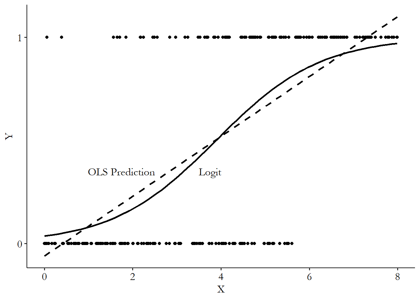
What do we see? As previously mentioned, we see the OLS prediction going outside the range of 0 and 1. But beyond that, the slopes of the OLS and logit models are different. This is especially true near the right or left sides of the graph. What does this mean? It means that the reason we were thinking about using OLS anyway - getting the effect of \(X\) on \(Y\) rather than caring about realistic predictions - falls apart anyway.
But why is this? Well, think about it - if \(X\) has a positive effect on \(Y\), but you already predict that \(Y\) has a .999 chance of occurring, then what should a one-unit increase in \(X\) do? Almost nothing, right? There’s simply not that much more that \(Y\) can increase by. But if your current prediction of \(Y\) is .5, then there’s a lot more room to grow, so the effect can be bigger. It should be bigger! OLS is unable to account for this.279 Even using a polynomial in OLS, while it would introduce a curvy line that might even look a bit like the logit line, can’t quite get this job done in a consistent way.
OLS is unable to account for how the effect of \(X\) on \(Y\) should differ. This works in a different way to how the effect differed when we talked about polynomials. The curviness shouldn’t be based on the value of \(X\), as it is with a polynomial, it should be based on the current predicted value of \(Y\). When the sample average of \(Y\) is in the middle - near .5 or so - using OLS isn’t a huge problem, although you still might want to use probit or logit anyway. But if the average of \(Y\) is anywhere near 0 or 1, you have a big problem and absolutely need a nonlinear model.
Interpreting a generalized linear model can be a little trickier than interpreting an OLS model. In one, very narrow and pretty useless sense, the interpretations are exactly the same. That is to say, each coefficient still means “a one-unit change in this variable is associated with a (coefficient-sized) change in the index.” That’s true whether we’re talking about linear or nonlinear regression. The difference, however, is that with OLS, the index function is just a regression equation giving us the conditional mean of the dependent variable, and we know how to interpret a change in the dependent variable.280 Technically, OLS doesn’t have a “link function,” although linear GLM does. But I think this is still a clear way to explain it so… let’s stick with it. In GLM, the index function is the thing that gets put through the link function. So it’s in terms of “units of change in the thing that gets put through the link function,” which is way harder to think about.
Marginal effect. In a probit or logit model, the effect/association of a one-unit change in a variable \(X\) on the probability that the binary dependent variable \(Y\) is 1/“true.”
It’s common to present the results of probit and logit models, and nonlinear regression more generally, in terms of their marginal effects. Marginal effects basically translate things back into linear-model terms. While the coefficient on \(X\) in a logit model gives the effect of a change in \(X\) on the index, the marginal effect of \(X\) gives the effect of a change in \(X\) on the probability that the dependent variable is 1.
Mathematically, the marginal effect is straightforward, although we do have to dip back into the calculus well once again. The marginal effect of \(X\) on the probability that \(Y = 1\) is just the derivative of \(Pr(Y = 1)\) with respect to \(X\), which has a conveniently simple solution for these binary-dependent variable models:
So the marginal effect of \(X\) is equal to the coefficient on \(X\), \(\beta_1\), multiplied by the predicted probability that \(Pr(Y = 1)\) (which comes from the model, and is conditional on all the predictor values) and one minus that same probability. Note that \(Pr(Y=1)(1-Pr(Y=1))\) is tiny when \(Pr(Y=1)\) is near 0 or 1, and at its biggest when \(Pr(Y=1) = .5\), so we retain the result from Figure 13.11 that the slope is steepest in the “middle” of the graph and flattest on the sides.
There is, however, a catch. That catch is that there is no one marginal effect for a given variable. I just said to look back at Figure 13.11. Well… keep looking at it! As \(X\) increases, the logit-predicted probability that \(Y = 1\) might go up by a tiny amount (on the left or right side of the graph) or by quite a bit (in the middle). In fact, each observation in the data has its own marginal effect, based on the \(Pr(Y=1)\) for that observation, as we’d expect based on the \(\beta_1Pr(Y=1)(1-Pr(Y=1))\) equation for the marginal effect. If the model predicts you’re 90% likely to have \(Y = 1\), your marginal effect is \(\beta_1(.9)(.1)\). If it predicts you’re 40% likely, your marginal effect is \(\beta_1(.4)(.6)\). So what value do we give as “the” marginal effect?281 Crucially, this variation in effect across the sample is not the same as treatment effect heterogeneity as we explored in Chapter 10 or when talking about interaction terms. The marginal effect varying with \(P(Y=1)\) only captures one narrow aspect of variation in the effect - only the part that has to do with “not having much room to grow” near the maximum or minimum \(Y\) predictions. Not to do with, say, a treatment being more effective for men than for women. All that treatment effect heterogeneity stuff applies in probit/logit models too, but you have to deal with it explicitly like you would in OLS.
There are two common approaches to this issue, one of which I will heavily recommend over the other. The first, which I will not recommend, is the “marginal effect at the mean.” The marginal effect at the mean first takes the mean of all the predictor variables. If we’re just working with \(X\), then it takes the mean of \(X\). Then, it uses that mean to predict \(Pr(Y=1)\). And finally it uses that predicted \(Pr(Y=1)\) to calculate the marginal effect, \(\beta_1Pr(Y=1)(1-Pr(Y=1))\). This gives the marginal effect of an observation with completely average predictors. Why don’t I recommend this? Because it’s calculating the marginal effect for no person in particular. Who is this marginal effect for, anyway?282 Statistics has no shortage of creating representative values that don’t actually represent any particular individual - that happens any time we use a mean. But in this case, there are other issues, too, and we have better options. The nobody-really-has-2.3-children problem isn’t enough of a problem to make us give up on means entirely, as means are invaluable for other reasons, but it can be enough to give up on marginal effect at the mean, which has superior alternatives. Plus, marginal effects at the mean take the mean of each variable independently, when really these variables are likely to be correlated. It’s strange to take the mean of everything, for example, if someone with a near-mean value of \(X\) almost always has a near-minimum value of \(Z\).
Average marginal effect. The mean of the calculated marginal effect across every observation in the sample.
What I recommend instead is the average marginal effect. The average marginal effect calculates each individual observation’s marginal effect, using that observation’s predictors to get \(Pr(Y = 1)\) and then \(\beta_1Pr(Y=1)(1-Pr(Y=1))\). Then, with each individual observation’s marginal effect in hand, it takes the average to get the average marginal effect. That’s it! Then you have the mean of the marginal effect across the sample, which gives you an idea of the representative marginal effect.283 Of course, nothing requires you to get the mean - you can do whatever you want with the effect distribution. Take the median, standard deviation, whatever. Or look at the whole distribution. But in general people focus on the mean here.
To take a quick example, let’s say we estimated the logit model \(Pr(Y=1) = logit(.1 + .05X - .03Z)\). And for simplicity’s sake let’s say we did this with only two observations in the sample. The first observation has \(X = 1\) and \(Z = 2\), and the second has \(X = 0\) and \(Z = 20\).
The predicted value for the first observation is \(Pr(Y = 1) = logit(.1 + .05(1) - .03(2)) = logit(.99) = \frac{e^{.99}}{1+e^{.99}} \approx .729\). Similarly, the predicted value for the second observation is \(Pr(Y = 1) = logit(.1 + 0 - .03(20)) = logit(-.5) =\frac{e^{-.5}}{1+e^{-.5}} \approx .622\). Then, the marginal effect of \(X\), since the coefficient on \(X\) is .05, would be \(.05(.729)(1-.729) = .010\) for the first observation, and \(.05(.622)(1-.622) = .012\) for the second. Average those out to get the average marginal effect of \((.010 + .012)/2 = .011\).
Let’s code up some probit and logit models! In the following code, I’ll show how to estimate a logit model, and then how to estimate average marginal effects for those models. What about probit? Conveniently, all of the following code samples can be used to estimate probit models, simply by replacing the word “logit” with the word “probit” wherever you see it.
In each case, we’ll be seeing whether weekend inspections have become more or less prevalent over time, once again with our restaurant inspection data.
In the case of the R code, you will often see guides online telling you to use the logitmfx function from the mfx package, instead of marginaleffects. This works fine, but do be aware that it defaults to the marginal effect at the mean instead of the average marginal effect.
R Code
# Load packages and data
library(tidyverse); library(modelsummary); library(marginaleffects)
df <- causaldata::restaurant_inspections

# Use the glm() function with
# the family = binomial(link = 'logit') option
m1 <- glm(Weekend ~ Year, data = df,
          family = binomial(link = 'logit'))

# See the results
msummary(m1, stars = c('*' = .1, '**' = .05, '***' = .01))

# Get the average marginal effect of year
avg_slopes(m1, variables = 'Year')
Stata Code
Python Code
import statsmodels.formula.api as smf
from causaldata import restaurant_inspections
df = restaurant_inspections.load_pandas().data

# smf.logit wants the dependent variable to be numeric
df['Weekend'] = 1*df['Weekend']

# Use smf.logit to run logit
m1 = smf.logit(formula = "Weekend ~ Year", data = df).fit()
m1.summary()
# And get marginal effects
m1.get_margeff().summary()
13.3 Your Standard Errors Are Probably Wrong
13.3.1 Why Your Standard Errors Are Probably Wrong
All of the things we’ve done with regression up to this point have been focused on getting our models right, setting up any nonlinearities properly, interpreting the coefficients, and, of course, identifying our effects. But the estimated model isn’t going to mean much for you if you don’t have some estimate of the precision of your estimates, i.e., a standard error (SE).284 I want to emphasize that standard errors really aren’t just for the purpose of calculating statistical significance! They give information about the sampling distribution of your estimate, which is good for lots of different approaches to using observed data to learn about theoretical/population distributions and relations.
As you’ll recall from earlier in the chapter, from estimating our model \(Y = \beta_0 + \beta_1X + \varepsilon\) we have our OLS coefficient estimate \(\hat{\beta}_1\) and our estimate of the standard error \(se(\hat{\beta}_1)\) (which we base on \(var(X), n\), and our estimate of \(\sigma\)). Then, our best guess for the sampling distribution of \(\hat{\beta}_1\) is a normal distribution with a mean of \(\hat{\beta}_1\) and a standard deviation of \(se(\hat{\beta}_1)\). This is the purpose of the standard error - it tells us about that sampling distribution, which lets us figure out things like the range of plausible estimates, confidence intervals, statistical significance, and eliminating certain theoretical/population distributions as unlikely.
That brings us to those error term assumptions I mentioned and said we’d come back to later. We want very badly to know what the sampling distribution is. We bother calculating the standard error because we want to know the standard deviation of that sampling distribution. But if certain assumptions are violated, then the standard error will not describe the standard deviation of the sampling distribution of the coefficient.
The first assumption we must return to is that we have to assume that the error term \(\varepsilon\) itself must be normally distributed.285 A common misconception is that the variables in the model must be normally distributed, but this is incorrect; we don’t need that. That assumption about the normality of the error term is what lets us prove mathematically that the OLS coefficients are normally distributed.
Conveniently, this assumption isn’t too important. OLS estimates tend to have sampling distributions pretty close to normal even if \(\varepsilon\) is pretty far from normal. Not perfect, but you don’t generally have to get too up in arms about this one. That said, there are some weird error-term distributions out there that really do mess things up. But that’s for another time.
The second assumption is that the error term is independent and identically distributed. That is, we need to assume that the theoretical distribution of the error term is unrelated to the error terms of other observations and the other variables for the same observation (independent) as well as the same for each observation (identically distributed). It doesn’t matter which data point you look at, the error term might be different from observation to observation, but it will always have been drawn from the same distribution.
What does this mean exactly? It’s easier to think about when it fails. One way it could fail is autocorrelation, where error terms are correlated with each other in some way. This commonly pops up when you’re working with data over multiple time periods (temporal autocorrelation) or data that’s geographically clustered (spatial autocorrelation).
Autocorrelation. When the error terms are correlated with each other.
Taking temporal autocorrelation as an example, say you’re regressing the US unemployment rate growth on year. The economy tends to go through up and down spells that last a few years, as in Figure 13.12. Think about the errors here - there tend to be a few positive errors in a row, then a few negative errors. So the distribution can’t be independent since the error from last period predicts the error this period.
Figure 13.12: US Unemployment Rate Over Time, with OLS Fit
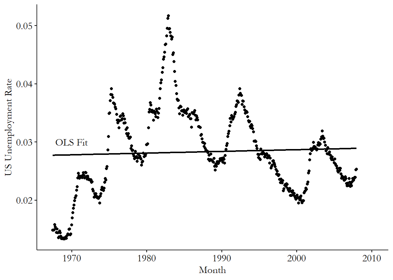
Another common way that being independent and identically distributed could fail is in the presence of heteroskedasticity. A big long word! Now this is a real textbook.
Heteroskedasticity. When the variance of the error term is related to the variables in a regression model.
Heteroskedasticity is when the variance of the error term’s distribution is related to the variables in the model. For example, say you were regressing how many Instagram followers someone has on the amount of time they spend posting daily. You might find that, as shown in Figure 13.13, among people who spend almost no time, there’s very little variation in follower count. But among people who spend a lot of time, there’s huge amounts of variation. Small amounts of time means little variation in follower count and, accordingly, little variation in the error term. But there’s a lot of variation in the error term for large amounts of time spent. The error distribution isn’t identical because the variance of the distribution changes with values of the variables in the model.
Figure 13.13: Simulated Instagram Follower Data
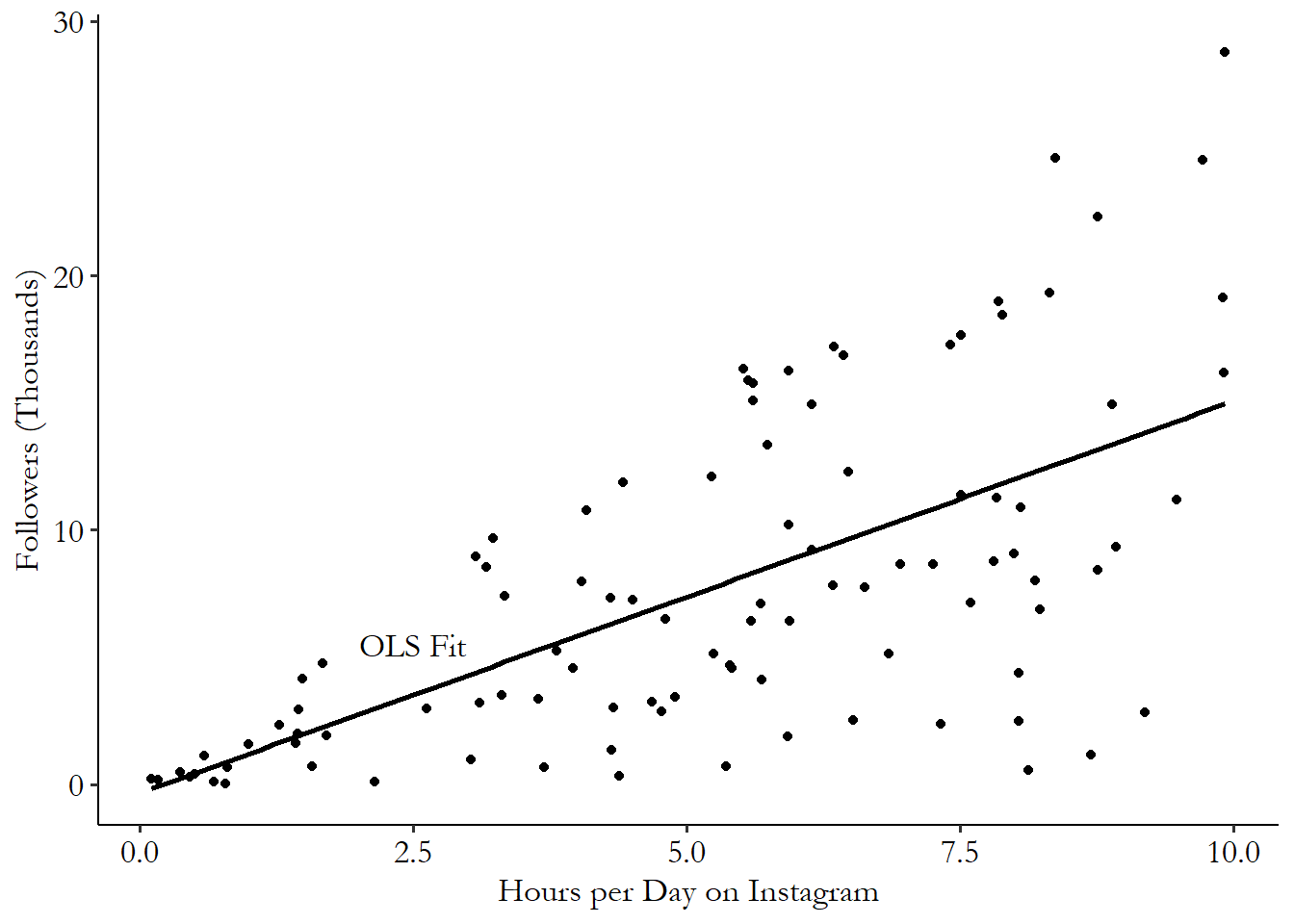
When it comes to failures of the “independent and identically distributed” assumption, we again have a convenient result. These failed assumptions don’t actually make the OLS coefficients non-normally distributed. However, they do make it so that our \(\sqrt{\sigma^2/(var(X)n)}\) estimate of the standard error is wrong. This means that we just have to figure out what the standard deviation of that sampling distribution is. This calculation will require some way of accounting for that autocorrelation or that heteroskedasticity.
13.3.2 Fixing Your Standard Errors
In this section I’m going to discuss a few common fixes to standard errors that we can use in cases where we think the independent and identically distributed assumption fails.286 Before getting too far into it, I want to point out that there are far more ways than these that standard errors can be wrong, and also more ways than these that they can be fixed. The Delta method, Krinsky-Robb… so many fixes to learn. Here I will show you only the beginning of the ways your standard errors will be wrong. If you decide to continue doing research, you can prepare for a lifetime of being wrong about your standard errors in fantastic ways that you can only dream of today.
First we’ll consider the issue of heteroskedasticity, which is when the variance of the error term \(\varepsilon\) changes depending on the value of \(X\) (or any of the predictors in the model, for that matter). The problem with heteroskedasticity, when it comes to estimating standard errors, is that in the areas where variance is higher, the conditional mean of \(Y\) in that area will move around more from sample to sample. Depending on whether this occurs for higher, lower, or middling values of \(X\), this might make \(\hat{\beta}_1\) change more from sample to sample (increasing the standard deviation of the sampling distribution) so as to meet those changing values. But since regular OLS standard errors simply estimate the same variance for the whole sample, it will understate how much things are changing.
To provide one highly simplified example of this in action, see Figure 13.14, which contains two data sets with the same level of overall error term variance across the sample. On the left, we have heteroskedasticity. Imagine picking one observation from the cluster on the left and one from the cluster on the right and drawing a line between them. That’s our OLS estimate from a sample size of 2. Now imagine doing it over and over.287 If you’re more of a physical learner, hold a pencil in your hands - the height of each hand is the conditional mean of \(Y\) in your sample, and the angle of the pencil as you hold it is \(\hat{\beta}_1\). Now move your hands up and down, independent of each other. Sometimes this changes the angle a lot - if the left hand goes up but righty goes down - but sometimes it doesn’t - if both go up. That’s regular sampling variation. Now try moving just one hand up and down. The angle changes much more rapidly! That’s one form of heteroskedasticity. With the \(Y\) value fairly pinned down on the right, but moving a lot on the left, the slope moves a lot from sample to sample - it’s that high-variance cluster driving this, which won’t be accounted for in the sample-wide estimate of the residual variance. Now do the same thing on the right. The slope is still going to vary from sample to sample, but the extent of this variation is driven by the variance in each cluster, which is the same, and so when we estimate that variation using the sample-wide residual variation, we’ll estimate it properly.
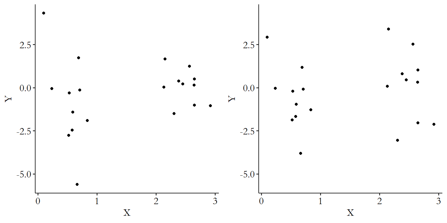
Figure 13.14: A Very Simplified Demonstration of Why Heteroskedasticity Messes up Standard Errors
Given this problem, what can we do? Well, we can simply have our estimate of the standard error personalize what we think about the error variance. Instead of \(\sqrt{\sigma^2/(var(X)n)}\) we can use a “sandwich estimator,” which, in short, allows the individual \(X\) values that go into that \(var(X)\) calculation to be scaled up, or down, or even be multiplied by other observations’ \(X\) values.288 It’s called a “sandwich estimator” because in the matrix-algebra form of the estimator, which is \((X'X)^{-1}(X'\Sigma X)(X'X)^{-1}\), the matrix \(\Sigma\) that does the scaling (and, later, lets the observations be correlated) gets “sandwiched inside” a bunch of \(X\)s.
One of the more common heteroskedasticity-robust sandwich estimator methods is Huber-White. In Huber-White, the scaling of the individual \(X\) values works by taking each observation’s residual, squaring it, and applying that squared residual as a weight to do the scaling. This, in effect, weights observations with big residuals more when calculating the variance.
There are actually several different estimators that, in very similar ways but with minor tweaks, adjust standard errors for the presence of heteroskedasticity. In general, you’re looking here for “heteroskedasticity-robust standard errors” or just “robust standard errors,” most of which are sandwich estimators, and with Huber-White standard errors as the classic application.289 Some users of regression, especially economists, tend to assume that heteroskedasticity is always a problem and so use heteroskedasticity-robust standard errors by default. I can’t say they’re wrong. However, an alternative to Huber-White called HC3 is generally considered a preferred improvement and the desired default option (Long and Ervin 2000Long, J. Scott, and Laurie H. Ervin. 2000. “Using Heteroscedasticity Consistent Standard Errors in the Linear Regression Model.” The American Statistician 54 (3): 217–24.), since it uses a “jackknife,” method for estimating the \(\Sigma\) in the sandwich.290 In a “jackknife” the model is estimated multiple times, each time dropping one of the observations, calculating variance by seeing how much the single dropped observation affects the estimate. HC3 performs about the same in big samples, but much better in small samples (MacKinnon and White 1985MacKinnon, James G., and Halbert White. 1985. “Some Heteroskedasticity-Consistent Covariance Matrix Estimators with Improved Finite Sample Properties.” Journal of Econometrics 29 (3): 305–25.). There are other versions besides Huber-White and HC3, to be applied in different scenarios, but these days HC3 is considered a very good place to start.
We can then move along to errors that fail to be independent. In other words, they’re correlated with each other. Why would correlated errors require us to change how we calculate standard errors? Correlated errors will change the sampling distribution of the estimator in the same way that correlated data would change a sampling distribution of a mean. Say you were gathering samples of people and calculating their height. If you randomly sampled people from all over the globe each time, that would give you a certain standard deviation for the sampling distribution of the average height. But if instead you randomly sampled families each time and calculated average height, the values would be correlated - your height is likely more similar to your parents than to some stranger. We’d be more likely than in the randomly-sample-everyone approach to get all tall people and thus a very tall average, or all short people and thus a very short average. So the mean is swingier, and the sampling distribution has a larger standard deviation. Some adjustment must be made.
When figuring out what adjustment to make, we’re in a bit of a pickle - we have to figure out how the errors correlated with each other. After all, it doesn’t make much sense to say “my errors are correlated” - they can’t all be correlated. Instead, we’d say they’re correlated according to some feature. Each of the different ways they can be correlated calls for a different kind of fix.
One common way in which errors can be correlated is across time - this is the time-based autocorrelation we discussed earlier. In the presence of autocorrelation we can use heteroskedasticity- and autocorrelation-consistent (HAC) standard errors.291 Autocorrelation-consistent standard errors are only one tool out of like a billion in the back pocket of anyone working with time series data. These tools are almost entirely absent from this book. While time series does pop up in a few places here, like in Chapter 17 on event studies, for a serious treatment of time series you’re better off looking at a more traditional econometrics textbook.
A common approach to HAC standard errors is the Newey-West estimator, which is another form of sandwich estimator. This estimator starts with the heteroskedasticity-robust standard error estimate, and then makes an adjustment.292 Why start with robust SEs? Why not just a fix for autocorrelation and not heteroskedasticity? Because autocorrelation by its nature tends to introduce heteroskedasticity anyway. If errors are correlated, then at times where one observation has a small error, other nearby observations will also have small errors, producing low error variance. But at times where one observation has a large error, other nearby observations will also have large errors, producing high variance. Low variance at some times and high variance at other times. Heteroskedasticity! That adjustment comes from first picking a number of lags - the number of time periods over which you expect errors to be correlated. Then, we calculate how much autocorrelation we observe in each of those lags, add them together - with shorter-length lags being featured more heavily in the sum - and that’s used to make the adjustment factor.293 In a bit more detail, we multiply the de-meaned time series by the error terms, and calculate the correlation between that and its lag. We sum up those correlations, weighting the one-period lag by just below 1, then with declining weights for further lags. Take that sum, multiply it by two, and add one. That’s the adjustment factor.
Autocorrelation across time is not the only form of autocorrelation, with correlation across geography also being highly consequential. While I won’t go deeply into the subject here, Conley spatial standard errors are another form of sandwich estimator, which calculates standard errors while accounting for the presence of autocorrelation among geographic neighbors.
Another common way for errors to be correlated is in a hierarchical structure. For example, say you’re looking at the effect of providing laptops to students on their test scores. Well, a given classroom of students isn’t just given laptops or not, they are also in the same classroom with the same teacher. Whatever we predict about their test scores based on having laptops, they’re likely to all be similarly above-prediction or below-prediction together because of the similar environments they face - their errors will be correlated with each other. We’d say these errors are clustered within classroom.
Conveniently, in these cases, we can apply clustered standard errors. The most common form of clustered standard errors are Liang-Zeger standard errors, which are again a form of sandwich estimator. With clustered SEs, you explicitly specify a grouping, such as classrooms. Then, instead of using the sandwich estimator to scale up or down individual \(X\) values, it instead lets \(X\) values interact with other \(X\) values in the same group.294 For the matrix algebra fans: remember that \(\Sigma\) matrix that’s “sandwiched between” all the \(X\)s from a few notes ago? Well, for clustered standard errors, this matrix is block-diagonal, where each grouping has unrestricted nonzero values within its block, but the rest of the matrix is 0. \(^,\)295 What’s the difference between including a control for a group indicator in the model, and clustering at that group level? First off, you can do both, and people often do. Second, including the indicator in the model suggests that group membership is an important predictor of the outcome and possibly on an important back door, while clustering suggests that group membership is related to the ability of the model to predict well.
The use of clustered standard errors can account for any sort of correlation between errors within each grouping.296 They can even be used to account for autocorrelation of any sort in panel data where you have multiple time series all in one data set - just cluster by the time series. This sort of flexibility is a nice relief. No need to make those restrictive assumptions about error terms having correlations of zero. Of course, statistical precision comes from assumptions. If you won’t assume anything, the data won’t tell you anything. So clustering at too broad a level (say, if your laptop-test score analysis has two schools and you cluster at the school level, or just clustering among the whole sample - everyone’s error is correlated with everyone else’s) is the equivalent of saying “uh… I dunno what’s happening here, could be just about anything I guess,” and you’ll get very large standard errors that might understate what your data can actually tell you. So at some point you’ve got to put your foot down on just how far that correlation is allowed to spread.
What’s the right level to cluster at, then? First off, if you have a strong theoretical idea of when errors should be clustered together, such as in a classroom, go for it. Beyond this, another common approach is to cluster at the level of treatment. So, in the laptop example, if laptops were assigned to some classrooms but not others, you’d cluster at the classroom level. But if they were assigned to some schools and not others, you’d cluster at the school level. Even then, you’d only want to cluster if the treatment effect varies across your clusters.[Abadie2017] These are not hard-and-fast rules, however, and clustering decisions require a lot of knowledge about the specific domain you’re working in. See if you can find other people working on your topic and figure out how they’re clustering. Also see further discussion of clustering in the How the Pros Do It section of Chapter @ref{ch-FixedEffects}.
Something important to remember about the Liang-Zeger clustered standard errors, though, is that they work really well for large numbers of clusters, say, more than 50. Fewer clusters than that and they’re still an improvement on regular standard errors, but they’re nowhere near as accurate as you want them to be.297 Or even if you have a lot of clusters, but treatment is assigned along cluster lines and you only have a few treated clusters. For smaller numbers of clusters, you may instead want to use wild cluster bootstrap standard errors, which are sort of a mix between clustered standard errors, which we’re discussing now, and bootstrap standard errors, which I’ll discuss in the next section. See more about wild cluster bootstrap standard errors in Chapter 15.
So is it just sandwiches all the way down? No! There’s another way of estimating standard errors that has very broad applications, and that’s bootstrap standard errors. The bootstrap is about as close to magic as statistics gets. What are we trying to do with standard errors? What’s the point of them? We want to provide a measure of sampling distribution, right? We want to get an idea of what would happen if we estimated the same statistic in a bunch of different samples.
So the bootstrap says: “let’s estimate the same statistic in a bunch of different samples and see what the distribution is across those samples. Ta-da! Sampling distribution.” Oh. Huh, that makes sense. Why didn’t we think of that at the start?
But hold on, how is it possible to estimate the statistic in a bunch of different samples? We only have the one sample! That’s the genius of the bootstrap. It uses the one sample we have, but resamples it. The process for a bootstrap is:298 I’m describing bootstrap standard errors here, but the concept of a bootstrap is broader than just standard errors, and you may see it pop up elsewhere. It’s certainly popular in machine learning.
- Start with a data set with \(N\) observations.
- Randomly sample \(N\) observations from that data set, allowing the same observation to be drawn more than once.299 Depending on the structure of the data - for example, in the context of panel data where the same individual is measured multiple times and so has multiple rows - it may make sense to not sample totally at random. The “cluster bootstrap,” for example, randomly samples chunks of data, perhaps individuals or groups rather than observations. This is a “bootstrap sample.”
- Estimate our statistic of interest using the bootstrap sample.
- Repeat steps 1-3 a whole bunch of times.
- Look at the distribution of estimates from across all the times we repeated steps 1-3. The standard deviation of that distribution is the standard error of the estimate. The 2.5th and 97.5th percentiles show the 95% confidence interval, and so on.
Does this actually work? Let’s take a very simple example. Four observations in our data: 1, 2, 3, 4, and we’re estimating the mean. The sample mean, of course, is \((1+2+3+4)/4 = 2.5\). The sample variance of the data is \(((-1.5)^2 + (-.5)^2 + (.5)^2 + (1.5)^2)/(4-1) = 1.67\). So the standard error that we’d calculate by our typical process is \(\sqrt{1.67/4} = .645\).
All right, now let’s try the bootstrap. We get our first bootstrap sample and it’s 1, 1, 4, 4 - remember, the same observation can be resampled, which means that some observations from the original data show up multiple times and others don’t show up at all. The mean of this bootstrap sample is \((1+1+4+4)/4 = 2.5\). We resample again and get 1, 3, 4, 4, with a mean of 3. Do it again! The next one is 1, 2, 4, 4, mean of 2.75. Next! 1, 2, 2, 3, mean of 2. So far the average of the bootstrap samples we’ve taken is \((2.5 + 3 + 2.75 + 2)/4 = 2.56\), and the standard deviation is .427.
.427 is not exactly the .645 that we know is correct, but we’re not anywhere near done. When you do a bootstrap, you generally want to do it hundreds if not thousands of times. Remember, we’re trying to mimic a theoretical distribution here by using real-world resampling. We’re going to want to get a bit closer to the theoretical infinite number of observations that the theoretical distribution is based on.
Let’s go a bit bigger. Instead of our observations being 1 to 4 let’s do 1 to 1,000, and we’ll calculate 2,000 bootstrap samples instead of four bootstrap samples. Now, our sample mean is 500.5, and the standard error of that mean calculated using the standard method is 9.13. The mean of our bootstrap distribution is 500.5 as well, and the standard deviation of our 2,000 bootstrap samples turns out to be 9.06.300 This exact number will be a bit different each time you do bootstrap since there is randomness in the process. If you do bootstrap and want your results to be replicable, be sure to set a random seed in your software before doing it. A bit smaller than 9.13, but we’re basically getting what we thought we’d get. This is showing us that maybe those theoretical-distribution assumptions were actually a little pessimistic about the precision in this particular instance.301 Remember, those theoretical distributions are only approximations as far as the actual data goes.
This is the basic process by which bootstrap standard errors can be calculated. A bit computationally intensive, definitely. But on the flip side, they can sometimes point out where the traditional estimates are too conservative (or not conservative enough), they let you explore any part of the sampling distribution you’re curious about - median, different percentiles, skew, etc., not just the standard deviation - and they are very useful in estimating standard errors for unusual stuff. What if we have an estimator that we’re not sure follows a normal distribution, or any distribution we know about? No problem! Just bootstrap it.
Bootstrap does come with its own set of assumptions and weaknesses, of course - it may be magic, but while there may be such a thing as magic there’s no such thing as a free lunch. The bootstrap doesn’t perform particularly well with small sample sizes,302 If you’re wondering why I switched from a sample of 4 to a sample of 1,000 for my example above, that’s why. it doesn’t perform well for “extreme value” distributions (super highly skewed data), and it has some difficulties that at the very least need to be addressed if the observations in the data are related to each other, for example in panel data where multiple observations represent the same individual over time. For another example, the standard bootstrap doesn’t do well under autocorrelation. But for an estimate with a decent sample size and some well-behaved independently-distributed data, the bootstrap can be a great option, especially if the regular standard errors are difficult to calculate in that context. Also, there are some alternate versions of the bootstrap discussed in Chapter 15 that address some of these problems.
Let’s put some of those standard error adjustments into action. In each of the following code samples, I will show first how to implement heteroskedasticity-robust standard errors, heteroskedasticity- and autocorrelation-consistent standard errors, and then clustered standard errors.
First, robust standard errors. We will continue to use our restaurant inspection data here.
One important thing to know about robust standard errors, especially when it comes to coding them up, is that there are actually many different ways of calculating them. Each method uses different minor adjustments on the same idea. Some versions work better on small samples; others work better on certain kinds of heteroskedasticity. All of the methods below provide access to multiple different kinds of robust estimators (often given names like HC0, HC1, HC2, HC3, and so on). But different languages select different ones as defaults.303 This leads to much confusion when trying to replicate your results from one language in another language. For example, Stata’s famously easy robust option unfortunately defaults to HC1, so we’ll need to instead use vce(hc3) to get the probably-should-be-default HC3. Most R methods default to HC3. Always be sure to check the documentation to see which one you’re getting, and think about which one you should use.
R Code
# Load packages
library(tidyverse)
# For approach 1
library(AER); library(sandwich)
# For approach 2
library(modelsummary)
# For approach 3
library(fixest)

df <- causaldata::restaurant_inspections

# In R there are many ways to get at robust SEs
# For the first two methods we'll look at, we need to estimate
# the regression on its own
# (most types of regressions will work, not just lm()!)
m1 <- lm(inspection_score ~ Year + Weekend, data = df)

# First, the classic way, sending our regression
# object to AER::coeftest(), specifying the kind
# of library(sandwich) estimator we want
# vcovHC for heteroskedasticity-consistent
coeftest(m1, vcov = vcovHC(m1))

# Second, we can take that same regression object
# and, do the robust SEs inside of our msummary()
msummary(m1, vcov = 'robust',
         stars = c('*' = .1, '**' = .05, '***' = .01))

# Third, we can skip all that and use a regression
# function with robust SEs built in, like
# fixest::feols()
feols(inspection_score ~ Year + Weekend, data = df, se = 'hetero')
# (this object can be sent to modelsummary
# or summary as normal)
Stata Code
Next, we will address autocorrelation using Newey-West standard errors. Keep in mind that in each case you must select a maximum number of lags (or have one be selected for you). This book doesn’t focus much on time series, so I won’t go that deeply into it. But basically, closely examine the autocorrelation structure of your data to figure out how far to let the lags go.
Because these are intended for use with time series data, we will first need to adjust our data to be a time series.
R Code
# Load packages
library(tidyverse)
# For approach 1
library(AER); library(sandwich)
# For approach 2
library(fixest)

df <- causaldata::restaurant_inspections

# Turn into a time series
df <- df %>%
  group_by(Year) %>%
  summarize(Avg_Score = mean(inspection_score),
            Pct_Weekend = mean(Weekend)) %>%
  # Only the years without gaps
  filter(Year <= 2009) %>%
  # feols requires an index to do this
  mutate(index = 1)

# Perform our time series regression
m1 <- lm(Avg_Score ~ Pct_Weekend, data = df)

# Use the same coeftest method from robust SEs, but use the
# NeweyWest matrix. We can set maximum lags ourselves,
# or it will pick one using an automatic procedure (read the docs!)
coeftest(m1, vcov = NeweyWest)

# Or just use feols from fixest
# Note that fixest applies a small-sample correction and
# uses a "classic" form of HAC that does not apply
# "pre-whiting", so results are different
feols(Avg_Score ~ Pct_Weekend, data = df,
      panel.id = ~ index + Year, vcov = 'NW')
Stata Code
causaldata restaurant_inspections.dta, use clear download

* Turn our data into a single time series
collapse (mean) weekend inspection_score, by(year)

* Only use the run of years without gaps
keep if year <= 2009

* Tell Stata we have a time series dataset
tsset year

* Use "newey" instead of "regress"
* We must set maximum lags with lag()
newey inspection_score weekend, lag(3)
Python Code
import statsmodels.formula.api as smf
from causaldata import restaurant_inspections
df = restaurant_inspections.load_pandas().data

# Get our data into a single time series!
df = df.groupby('Year').agg({'inspection_score': 'mean',
'Weekend':'mean'})
# Only use the years without a gap
df = df.query('Year <= 2009')

# We can simply add cov_type = 'HAC' to our fit, with maxlags specified
m1 = smf.ols(formula = 'inspection_score ~ Weekend',
            data = df).fit(cov_type = 'HAC',
            cov_kwds={'maxlags':1})
m1.summary()
# Note that Python uses a "classic" form of HAC that does not apply
# "pre-whiting", so results are often different from other languages
For the last of our sandwich estimators, we can use clustered standard errors. We don’t really have any grouping that makes a whole lot of sense to cluster by in the data. But since this is only a technical demonstration, we can do whatever. We’ll be clustering by whether the inspection was on a weekend. There are only two values of this, which is not a lot of clusters. We could get some strange results.
R Code
# Load packages
library(tidyverse)
# For approach 1
library(AER); library(sandwich)
# For approach 2
library(modelsummary)
# For approach 3
library(fixest)

df <- causaldata::restaurant_inspections

# In R there are many ways to get at clustered SEs. For the first
# two methods we'll look at, we need to estimate the regression on
# its own. (most commands will work, not just lm()!)
m1 <- lm(inspection_score ~ Year + Weekend, data = df)

# First, the classic way, sending our regression object to
# AER::coeftest(), specifying the kind of library(sandwich) estimator.
# We want vcovCL for clustering.
# Note the ~ before Weekend; this is technically a formula
coeftest(m1, vcov = vcovCL(m1, ~Weekend))

# Second, we can pass it to msummary which will cluster if we send
# a formula with the cluster variable to vcov
msummary(m1, vcov = ~Weekend,
         stars = c('*' = .1, '**' = .05, '***' = .01))

# Third, we can use a regression function with clustered SEs built in,
# like fixest::feols(). Don't forget the ~ before Weekend.
feols(inspection_score ~ Year + Weekend,
    cluster = ~Weekend,
    data = df)
Stata Code
Python Code
import statsmodels.formula.api as smf
from causaldata import restaurant_inspections
df = restaurant_inspections.load_pandas().data

# We can simply add cov_type = 'cluster' to our fit, and specify the groups
m1 = smf.ols(formula = 'inspection_score ~ Year',
            data = df).fit(cov_type = 'cluster',
            cov_kwds={'groups': df['Weekend']})

m1.summary()
Finally, we come to bootstrap standard errors. There’s a necessary choice here of how many bootstrap samples to make. So… how many should you make? There’s not really a hard-and-fast rule. For most applications, a few thousand should be fine. So let’s do that. The code below only shows a straightforward each-observation-is-independent bootstrap. But in general something like a cluster boostrap, where certain observations are all included or excluded together, isn’t far off if you read the documentation, or Chapter 15.
R Code
# Load packages and data
library(tidyverse); library(modelsummary); library(sandwich)
df <- causaldata::restaurant_inspections

# Let's run our standard model from before
m <- lm(inspection_score ~ Year + Weekend, data = df)

# And use the vcov argument of msummary with vcovBS from the
# sandwich package to get boostrap SEs with 2000 samples
msummary(m, vcov = function(x) vcovBS(x, R = 2000),
         stars = c('*' = .1, '**' = .05, '***' = .01))
Stata Code
Python Code
import pandas as pd
import numpy as np
import statsmodels.formula.api as smf
from causaldata import restaurant_inspections
df = restaurant_inspections.load_pandas().data

# There are bootstrap estimators in Python but generally not designed for OLS
# So we'll make our own. Also see the Simulation chapter.
def our_reg(DF):
    # Resample with replacement
    resampler = np.random.randint(0,len(df),len(df))
    DF = DF.iloc[resampler]

    # Run our estimate
    m = smf.ols(formula = 'inspection_score ~ Year',
               data = DF).fit()
    # Get all coefficients
    return(dict(m.params))

# Run the function 2000 times and store results
results = pd.DataFrame([our_reg(df) for i in range(0,2000)])
# Mean and standard deviation are estimate and SE
results.describe()
13.4 Additional Regression Concerns
All that and we still aren’t done with regression? How long is this chapter?304 And if you’re tired of reading it, think about how I feel writing it. This chapter is topping 30,000 words - novella length! My fingers are tired. But I must press on. You WILL understand linear modeling. Oops, wait, hold on. My ring finger fell off. Alas, as with any statistical method, there are infinite little crevices and crannies to look into and wonder whether the method is truly appropriate for your data. And for something as widely-used as regression, it’s worth our time to explore what we can.
In this final section we’ll look at four additional tricks or concerns we’ll want to keep in mind when working with regression.
13.4.1 Sample Weights
Everything we’ve said about using a sample relationship to learn about a population relationship makes the assumption that the sample is drawn randomly from that population. So if we have a sample of, say, Brazilians, then each person in Brazil is equally likely to end up in our sample, whether they live in Rio de Janeiro or the countryside, whether they’re rich or poor, whether they’re educated or not, and so on.
This is rarely true for a number of reasons. Some people are easier to survey or gather data on than others. Some sampling methods don’t even try to randomly sample everyone, instead sampling people based on convenience, or location, or any number of other characteristics.
When this occurs, obviously, the results are better-representative of the people who were more likely to be sampled. We can solve this issue with the application of sample weights, where each observation in the sample is given some measure of importance, with some observations being treated as more important (and thus influential in the estimation) than others.
Sample weight. A scaling applied to each observation when calculating sample statistics.
In application to a bivariate regression, our estimate of the slope is \(Cov(X,Y)/Var(X)\). Without a sample weight, we estimate the covariance by taking \(X - \bar{X}\) and multiplying it by \(Y - \bar{Y}\) for each observation, then taking the average of that product over all the observations. With a sample weight \(w\), we do the exact same thing, but we take our \((X-\bar{X})(Y-\bar{Y})\) for each observation and multiply that by the observation’s weight \(w\) before taking the average of that whole thing.305 Often the weight will be standardized so the average of all weights over the whole sample is 1. This prevents the estimate from, say, calculating an overall bigger variance rather than just a variance that better-represents some observations. Also, formally what’s happening here is that every value of every variable is being multiplied by \(\sqrt{w}\). Then when you multiply two variables together, as in \(XY\) for the covariance, or \(XX\) for the variance, that becomes the weight \(\sqrt{w}^2 = w\). The higher your \(w\), the more your values will count when calculating the covariance, variance, and so on, and so you’ll be more represented in the final estimates.
This whole process is known, unsurprisingly, as weighted least squares.
Weighted least squares. Ordinary least squares performed with sample weights.
There’s more than one reason to weight. The problem I just mentioned - where certain people are more likely to be sampled than others - is a very common problem in the social sciences. It’s so common, in fact, that many surveys, and certainly most of the big and well-performed surveys like the census in most countries, will contain sample weights already prepared for you. The survey planners have a good idea about how their sampling was done, and so have a decent idea of how likely different individuals, households, firms, or whatever, were to be included in the sample.
These weights are sometimes created by comparing the proportion of people with a given attribute in the data against a population value. If the population has 500 men and 500 women (50% of each), and our sample of 100 people has 70 men and 30 women, then we might say that each man had a \(70/500 =\) 14% chance of being included, and each woman had a \(30/500 =\) 6% chance. Those probabilities would inform our sample weights.
Then, we’d weight each individual by the inverse of those probabilities. So men would get a \(1/.14 \approx 7.143\) weight, and women would get a \(1/.06 \approx 16.667\) weight. This weights people who were less likely to be sampled more heavily, giving us back the demographic proportions in the population, making our estimates better represent the population.
Inverse sample probability weights. A sample weight where each observation is weighted by the inverse of the probability that it was included in the sample.
For example, if we estimated the proportion of men using our sample alone, we’d estimate that the population has 70% men. Clearly wrong! But if we weight it, we’d get \((7.143\times70 + 16.667\times0)/(7.143\times70 + 16.667\times30) =\) 50%.306 That denominator (the \(7.143\times70 + 16.667\times30\)) is the sum of all the weights in the sample, and is there to scale the weights so they average out to 1. Perfect! Same idea goes when estimating regression coefficients. Without the weights, they’re skewed by the sampling process. With weights, we better represent the relationship in the population.
Sample weights work. If your data has sample weights (and they’re estimated properly, which in a professional survey they likely would be), read carefully about what they mean, and use them. Be sure to use the ones that fit the analysis you’re doing - survey data will often have different weights for different observation levels. If you want to generalize to individuals, use the individual-person weights. If you want to generalize to households use the household weights, and so on.
There are other reasons to weight, though. A big one comes if you’re using aggregated data. For example, maybe you’re doing an analysis of the impact of distributing laptops on test scores. But instead of using data on the individual students and their individual test scores, maybe you use classroom averages.307 In many real-world cases, you might only have access to the data on classroom averages. If you do have the individual data, often that’s what you want to use.
Now, analyzing the classroom-average data directly would have some problems. Some classrooms are bigger than others. Bigger classrooms represent more students, so if you want a result of the form “a laptop increases a student’s scores by \(\hat{\beta}_1\),” then your aggregated analysis will be hard to figure out, since your results would really be on the classroom-average level. Second, whatever average data you have will be less noisy if it came from a bigger classroom, since the sampling distribution of the mean has a smaller standard deviation if it comes from a bigger sample. So some of the means in your data will be better-estimated than others, but OLS will treat them as the same.
These are two different problems with two different (but similar) solutions.
Frequency weights. A sample weight equal to the number of observations represented in aggregated data, used so that the interpretation is on the non-aggregated level.
The first problem, and solution, is very simple. What if one classroom represents 30 people while another represents 40? Easy! Just count the first classroom 30 times and the second classroom 40 times. These are frequency weights, where the weight is simply the number of observations the variable represents. This returns your results to being interpretable on the individual, non-aggregated level. It’s not quite as good as actually having the non-aggregated data,308 Unless each observation in the group is, truly, exactly the same. since you lose out on that between-individual variation. But it does give you easier interpretation, and gives you a result that accounts for differences in size.
The second problem, relating to differences in the variance of the mean, is a bit trickier, but not much. For this problem we have inverse variance weighting. We can calculate the variance of each aggregated observation’s mean. Then, weight each observation by the inverse of that variance.
The variance of a sample mean is \(\sigma^2/N\), where \(N\) is the number of observations in the sample, i.e., the number of observations aggregated into the observation. The inverse of that is \(N/\sigma^2\). Under the assumption that \(\sigma^2\) is constant across the sample, that part drops out of the weighting (since it applies to everyone, and the weights are all relative to each other), leaving us with weights of \(N\). Each aggregate observation is weighted by the number of observations that got aggregated into it.
Hold on… frequency weights weight by the number of observations used to aggregate, too. So what’s the difference between frequency weights and inverse variance weights? There actually isn’t a difference when it comes to estimates - frequency weights and inverse variance weights will produce the exact same coefficients. However, there is a difference when it comes to standard errors. Frequency weights act as though each aggregated observation is truly a collection of separate, independent, completely identical observations. So when it calculates \(\sigma/var(X)\) for the standard errors, it uses the unaggregated sample size to calculate \(\sigma\). Inverse variance weights, however, recognize its data as being a set of means, and so uses the aggregated sample size to calculate \(\sigma\). Frequency weight standard errors will then always be smaller than inverse variance weight standard errors.309 So be really sure that “a collection of independent, completely identical observations” describes your data before using frequency weights. An example of this would be a randomized experiment with a binary outcome, so your four aggregated observations are “no treatment, \(Y = 0\),” “no treatment, \(Y = 1\),” “treatment, \(Y = 0\),” and “treatment, \(Y = 1\),” which would truly represent collections of independent observations.
Inverse variance weighting has plenty of other applications too, besides aggregated data. There are lots of other situations in which we know that some observations represent a lot more variance than others. For example, treatment itself may be a lot more variable for some observations than others, and those observations will be weighted more heavily in the estimate, which we can correct by inversing that variance to make the weight. Problem solved. One application of this to the fixed effects method can be seen in Chapter 16.
Another place where inverse variance weighting pops up that we won’t have room to cover is in meta-analysis. In meta-analysis, you look at a bunch of different studies of the same topic and try to estimate the overall effect, aggregating together their results. Some studies have estimates with big standard errors, and others have estimates with small standard errors. Inverse variance weighting helps weight the more precisely-estimated effects more strongly.
Let’s estimate some regressions with sample weights. Most commands will let you just give them a weighting variable. The task of figuring out which kind of weighting to do is on you, and you just pass off the final weight. So if you want inverse sampling probability weights, better calculate that inverse yourself!
This also means that if a certain approach to weighting requires you to adjust the standard errors, that won’t happen. If you want to do frequency weights, for example, you’ll either need to adjust the standard errors yourself, or skip the use of weights altogether and just copy each observation a number of times equal to its weight and run the regression without weights. You can do this in R by passing the data df to slice(rep(1:nrow(df), weight)) after loading the tidyverse.
Python is a bit trickier - you can do it with expanded_df = df.loc[numcopies], but this requires you to calculate numcopies, the number of times you want to copy each row, yourself. The itertools package may help with that.
Stata is an exception here, since it has several weight types (aweight, fweight, iweight, pweight) that it treats differently, and not all commands accept all kinds of weights. You’d generally use pweight for inverse-sampling-probability weights, aweight for variance weighting, and fweight for frequency weighting, which will properly handle the standard error adjustment for you.310 Although you could also do the copy-each-observation approach like with R and Python by using expand weight. Look at Stata’s help weight before using weights in Stata.
For these examples, we’ll be doing some inverse variance weighting with an aggregated version of our restaurant inspection data. First, we’ll aggregate the data to the different restaurant chains, and count how many inspections we’re averaging over. Specifically, we’ll see if average inspection score is related to the first year that the chain shows up in the sample. Then, since the variance of the sample mean is proportional to the inverse of the number of observations in the sample, we’ll weight by the inverse of that inverse, i.e., the number of observations in the sample.
R Code
# Load packages and data
library(tidyverse); library(modelsummary)
df <- causaldata::restaurant_inspections

# Turn into one observation per chain
df <- df %>%
    group_by(business_name) %>%
    summarize(Num_Inspections = n(),
    Avg_Score = mean(inspection_score),
    First_Year = min(Year))

# Add the weights argument to lm
m1 <- lm(Avg_Score ~ First_Year,
         data = df,
         weights = Num_Inspections)

msummary(m1, stars = c('*' = .1, '**' = .05, '***' = .01))
Stata Code
causaldata restaurant_inspections.dta, use clear download

* Aggregate the data
g Num_Inspections = 1
collapse (mean) inspection_score (min) year ///
    (sum) Num_Inspections, by(business_name)

* Since we want inverse-variance weights,
* we use aweights, or aw for short
reg inspection_score year [aw = Num_Inspections]
Python Code
import statsmodels.formula.api as smf
from causaldata import restaurant_inspections
df = restaurant_inspections.load_pandas().data

# Aggregate the data
df['Num_Inspections'] = 1
df = (df
.groupby('business_name')
.agg({'inspection_score': 'mean',
    'Year': 'min','Num_Inspections': 'sum'}))

# Here we call a special WLS function
m1 = smf.wls(formula = 'inspection_score ~ Year',
            weights = df['Num_Inspections'],
            data = df).fit()
These code examples, of course, just show how to run a single regression with weights. If you are working with survey data that has complex weighting structures that you’ll need to reuse over and over again, you might want to have the language explicitly acknowledge that and help you. In R you can do this with the survey package. In Stata you can look at the range of svy commands and prefixes with help svy and help svyset.
13.4.2 Collinearity
When I discussed categorical predictor variables, I talked about perfect multicollinearity. Perfect multicollinearity is when a linear combination of some of the variables in the model perfectly predicts another variable in the model. When this happens, the model can’t be estimated. If the model is \(Sales = \beta_0 + \beta_1Winter + \beta_2NotWinter\), then \(\beta_0 = 15, \beta_1 = -5, \beta_2 = 0\) produces the exact same predictions (and residuals) as \(\beta_0 = 10, \beta_1 = 0, \beta_2 = 5\), as well as an infinite number of other sets of estimates. OLS can’t pick between them. It can’t estimate the model.311 In practice, regression software will estimate the model, but only by dropping one of the variables so the perfect multicollinearity goes away.
But what happens if we don’t have perfect multicollinearity, but we do have predictor variables that are super highly correlated? After all, one way of thinking about \(Winter\) and \(NotWinter\) is they’re just two variables with a correlation of -1. What if we had two variables with a correlation of .99$ or -.99 instead of 1 or -1? Or even .9 or -.9? We’d call that a high degree of collinearity (but not perfect).
Collinearity. When a predictor variable in the model is very strongly predicted by a linear combination of the other variables in the model.
Outside of the categorical-variable example, high collinearity often comes up when you have multiple variables that measure effectively the same thing. For example, say you wanted to use an “Emotional Intelligence” score to predict whether someone would get a promotion. You give people an emotional intelligence test with two halves with tiny variations on the same questions. Then, you use the first half of the test and the second half as separate predictors in the model, hoping to get an overall idea of how emotional intelligence as a whole predicts promotions. The scores from those two halves are likely highly correlated.312 And if they’re not, that test probably isn’t very good.
High levels of collinearity tend to make the estimates very sensitive and noisy, leading the sampling distributions to be very wide and driving the standard errors upward.
Why does collinearity increase standard errors? Let’s stick with our Winter/Sales example. Let’s replace the Winter variable with WinterExceptJan1. So now our predictors are WinterExceptJan1, which is 1 for all non-January 1 days in Winter, and NotWinter, which is 1 for all non-Winter days. January 1 is zero for both of them. The correlation between the two variables would be very nearly -1. \(WinterExceptJan1 + NotWinter = 1\) is true for all observations except for January 1. So we are close to a perfect linear combination but not quite.
In that setting, with the model \(Sales = \beta_0 + \beta_1WinterExceptJan1+ \beta_2NotWinter\), \(\beta_0 = 15, \beta_1 = -5, \beta_2 = 0\) will not produce the exact same predictions (and residuals) as \(\beta_0 = 10, \beta_1 = 0, \beta_2 = 5\), but it will be very close. Every day but January 1 will be predicted exactly the same. Now, unlike with perfect multicollinearity, we can pick a “best” set of estimates. Simply set \(\beta_0\) equal to \(Sales\) on January 1, \(\beta_1\) equal to the average difference between \(Sales\) on the other Winter days and on January 1, and \(\beta_2\) equal to the average difference between \(Sales\) on non-Winter days and on January 1.
However, those estimates we picked were entirely dependent on the January 1 value. If Sales on January 1 are 5, then we get \(\beta_0 = 5, \beta_1 = 5, \beta_2 = 10\). If \(Sales\) on January 1 just happens to be 15 instead, then everything changes wildly to \(\beta_0 = 15, \beta_1 = -5, \beta_2 = 0\). A single observation changing value shifts every coefficient by about the amount of the shift! \(\beta_1\) then moves around just as much as a single observation of \(Sales\) does. The standard error of \(\beta_1\) basically is the standard deviation of \(Sales\), rather than shrinking quickly with the sample size as it normally would.313 This particular result is based on this very specific example of two categories with only one observation left out, but the same general idea applies to any kind of high-collinearity situation.
What can we do about collinearity then? The first step is, as always, to think through our model carefully. Even before thinking about whether a calculated correlation is really high, ask yourself “why am I including these predictors in the model?” Remember, adding another predictor to the model means you’re controlling for it when estimating the effect of the other variables. Do you want to control for it?
A tempting thought when you have multiple measures of the same concept is that including them all in the model will in some way let them complement each other, or add up to an effect. But in reality it just forces each of them to show the effect of the variation that each measure has that’s unrelated to the other measures.
Going back to the example with the two halves of the emotional intelligence test, why would we want to know the effect of the first half while controlling for the second half? “Controlling for the second half of the exam, an additional point on the first half increases…” what would that even mean? The coefficient on the first half would represent the relationship between score on the first half and promotion probability after removing the part of that relationship that’s explained by the second half, but that explained part should basically be all of the relationship. There won’t be much variance left, making \(var(X)\) tiny and \(\sigma^2/var(X)\) big, inflating those standard errors. In any case, where the correlation really is that strong, you probably aren’t closing any back doors, you’re just controlling away your treatment.
In cases like this, where we have multiple measures of the same thing, one good approach to including all the predictors while avoiding collinearity is the use of dimension reduction methods, which take multiple measures of the same thing and distill them down into their shared parts, capturing the underlying concept you think they all represent (rather than their non-shared parts, which is what including them all in a regression would do).
Dimension reduction is a large field, largely growing out of psychometrics, and I won’t even try to do it justice here. But methods like latent factor analysis and principal components analysis take multiple variables and produce a small set of factors that represent different shared aspects of those variables, either looking for components that are unrelated to each other (and so produce no collinearity at all), or instead focusing on getting those underlying concepts which might be related to each other. Unsurprisingly, machine learing researchers, who often have to deal with thousands upon thousands of variables at once, have also made a lot of contributions in recent years to dimensionality reduction. See Jia et al. (2022Jia, Weikuan, Meili Sun, Jian Lian, and Sujuan Hou. 2022. “Feature Dimensionality Reduction: A Review.” Complex & Intelligent Systems 8 (3): 2663–93.) for a review.
How can we address collinearity in other contexts, where the issue isn’t multiple measures of the same thing, but multiple measures of different things that happen to be strongly correlated?
For example, maybe you want to look at the impact of an increase in wages on a firm’s profitability, controlling for stock market indices in both Paris and Brussels, where it trades a lot. Paris and Brussels stock prices are likely correlated strongly, but they’re not the same thing. We can imagine how we might want to control for both, but maybe the correlation is too high and we’d have a collinearity problem. Should we remove one, or use dimension reduction? How much correlation is “too much”?
You could just check the correlation between all the predictors and seek out high correlations, but this wouldn’t account for cases where it takes more than one variable to form a very close linear prediction of a variable.
A common tool in checking whether there’s too much collinearity,314 In a linear regression, anyway. which takes into account the entire set of variables at once, is the variance inflation factor (VIF). The VIF is different for each variable in the model. Specifically, for variable \(j\), it’s \(VIF_j = 1/(1-R_j^2)\), where \(R_j^2\) is the \(R^2\) from a regression of variable \(j\) on all the other variables in the model.
As a very rough rule of thumb, if a variable has a VIF above 10 (i.e., if regressing that variable on the other predictors produces an \(R^2\) above .9), then you might want to consider removing it from the model, or performing dimension reduction with the other variables it’s strongly related to. Other people use a VIF above 5 as a cutoff. In general, using hard cutoffs as decision rules rarely makes sense in statistics. Instead, use high VIFs as an opportunity to think very carefully about your model and think about whether removing things makes sense.
You can calculate the VIF for each variable in the model in R using vif(m1) from the car package, where m1 is your model. In Stata, run your regression, and then follow that with estat vif.
Python has the variance_inflation_factor function which you can import from statsmodels.stats.outliers_influence. However, it works a bit differently from the R and Stata versions because it operates on a data frame of the predictors instead of on the model, and only calculates the VIF for one of them at a time, so you have to loop through them if you want everything. If X is a data frame consisting only of your predictors, you can calculate the VIF for each of them with [variance_inflation_factor(X.values, i) for i in range(X.shape[1])].
13.4.3 Measurement Error
It seems like a pretty reasonable assumption that the variables in the data are the variables in the data. But what if… they’re not?
What I mean by this is that it’s pretty common for the values you’ve recorded in the data to not be perfectly precise. It’s also common for the variable you have in the data to only be a proxy for the variable you want, rather than the real thing.
Imprecision is a natural part of life. No measurement is perfectly precise. If you have a data set of heights, the “5 foot 6 inch” and “6 foot 1 inch” in the data probably are hiding more accurate values like “5.5132161 feet” and “6.0781133 feet” that you don’t have access to. If the only problem is that you’ve rounded your values to a certain reasonable level of precision, that’s probably not a huge issue. But if the mismeasurement is more severe - if you’re rounding both of those very-different heights to 6 feet, or if that “5 foot 6 inch” is really “5 foot 8 inch” but someone wrote it down wrong, or used the ruler incorrectly, then the values in the data don’t match the real values, so there’s no way for our estimates to pick up on actually-existing values in the data.
Proxy. A variable that should be strongly related to the variable you actually want in your model, used in its place because you don’t have measurements of the variable you actually want.
The use of proxies is common as well. A proxy is a variable used in place of another, because you don’t have the variable you actually want. If you want to know the effect of giving students laptops on future test scores, you may think that mathematical ability exists on a back door and so want to control for a student’s mathematical ability. You can’t actually see their mathematical ability, but you have access to their scores on a math test, which isn’t exactly the same thing but should be closely related. The test score is a proxy for mathematical ability, but it’s not the same thing. If two students have the same ability but different test scores, the model will treat them as different when really they’re the same, and thus will get it wrong.
Measurement error. When a variable you’re using is an inexact representation of the variable you actually want, due to mismeasurement, imprecision, or using a proxy.
Latent value/latent variable. A value or variable that is a part of your model, but not a part of your data. Generally the term is only used when you have other variables you’re trying to use to represent the latent variable.
Imprecision and proxies are both examples of measurement error, also known as errors-in-variables. The idea is that the variables in your model represent the true latent value you want, with some error.
where \(X\) is the variable you have in your data, \(X^*\) is the latent unobserved variable, and \(\varepsilon\) is an error term.315 This equation shows the error term as being added to the true value, but it could easily work in some other way, for example being multiplied by the true value.
Why do we care about measurement error? It’s pretty easy to imagine how measurement error can lead our estimates astray. In the extreme, imagine using some completely unrelated variable as a proxy. If I want to know the effect of laptops on test scores, but instead of using the variable “has a laptop” I use “has brown hair,” we have no reason to believe that would give us the effect of having a laptop.
But what about in less extreme cases? There are two main kinds of measurement error, and they have different implications.
The easiest kind of measurement error to handle is classical measurement error, which is measurement error where the error \(\varepsilon\) is unrelated to the latent variable \(X^*\). When this happens, the measured variable \(X\) is just “the true latent variable, plus some noise.”
Classical measurement error has clear implications: in the regression \(Y = \beta_0 + \beta_1X\), if \(X\) suffers from classical measurement error, then the estimate \(\hat{\beta}_1\) will be closer to 0 than the true \(\beta_1\) you’d get if you could run \(Y = \beta_0 + \beta_1X\).316 This is also true in a model with controls. It will “shrink towards zero,” also called “attenutation.”
Why does it do this? Well, \(X^*\) has an effect of \(\beta_1\) on \(Y\), right? Whenever \(X^*\) moves, we expect \(Y\) to move as well. But if we see \(X\), the noisy version of \(X^*\), then we won’t see all those \(X^*\) moves. We’ll see \(Y\) dancing around, responding to changes in \(X^*\) that we can’t see in \(X\). And the more changes in \(Y\) there are that aren’t related to \(X\), the less related \(X\) and \(Y\) appear to be. So the estimate shrinks towards zero.
Classical measurement error also has some clear fixes, or, rather, it offers the opportunity not to fix it. Most commonly, people will just run regular OLS without actually fixing anything, and then treat the estimate as a “lower bound.” They know the effect is at least as far away from zero as the estimate they get, although they don’t know how much larger.
You may have noticed that I’ve only discussed measurement error in \(X\). What about \(Y\)? Turns out classical measurement error in \(Y\) just isn’t much of a problem. Sure, it will reduce the model’s \(R^2\) (since there’s now some more noise in \(Y\) that we can’t predict), but it won’t affect the coefficients, at least not on average. Those coefficients are already used to there being noise in \(Y\) it can’t predict. There’s just a bit more of it now. That noise will go into the regression model’s error term.
If that’s classical measurement error, what’s non-classical measurement error? This is when the error is related to the true value, and it makes things much trickier. Why might measurement error be non-classical? One example is if \(X^*\) is binary, as is \(X\), so both can only be 0 or 1. If \(X^* = 1\), then the error can only possibly be 0 or -1. If \(X^* = 0\), then the error can only possibly be 0 or 1. The value of \(X^*\) determines what the error can be, making them related.
Non-classical measurement error occurs with continuous variables, too. Say you have a bunch of tax data on business owners and are measuring income. You know that some people are going to misrepresent their income on their taxes, so as to pay less in tax. Misrepresenting income is a lot easier with cash-based businesses than with businesses that mostly get paid with credit cards or checks. Cash-based businesses also on average tend to have lower incomes than others. So we’d expect more negative measurement errors (underreported income) among low-income businesses than high-income businesses. The error is related to the true value.
For another example, imagine a study that relies on a variable where people report how much they exercise each day. Someone who exercises a lot may feel comfortable reporting the truth to the survey-taker, while someone who exercises very little may bump their numbers up to look better.
Non-classical measurement error is more unpredictable than classical measurement error, because without knowing more about the exact way the error is related to \(X^*\), we don’t know whether \(\beta_1\) will be shrunk toward zero, inflated away from zero, biased upward, biased downward, or not biased at all! It could be anything. Also, unlike classical measurement error, non-classical measurement error is a problem when it happens to \(Y\) as well as when it happens to \(X\).
So if you think you have measurement error, put some serious thought into whether you think there’s any way for that error to be related to the latent variable. If it is, you have a bigger problem on your hands than you thought.
If we have measurement error and want to fix it, how can we do that? If you have some information about the measurement error itself, you might be able to do some adjustments to get closer to the true \(\beta_1\). I won’t go deeply into these methods - you’ll have to look elsewhere. Measurement error is one of those topics where diving in takes you really deep. Every textbook I can find focusing on the subject is much more advanced than the one you’re reading now, but it still may be worth your time to look at a book like Measurement Error Models by Wayne Fuller (2009Fuller, Wayne A. 2009. Measurement Error Models. Vol. 305. John Wiley & Sons.).
Without going too deep, though (or, rather, rattling off the keywords you can Google for later), what can we do? If you have an idea of the ratio of the variance of the regression error to the variance of the measurement error, you can perform a Deming regression or Total Least Squares, which adjusts for the shrinkage towards zero.
There are other options out there that you can look for, including the general method of moments (GMM). Another common approach is the use of instrumental variables, although unlike with the use of instrumental variables in Chapter 19, the goal here is not to identify a causal effect but rather adjust for measurement error. If you have two measurements of the same latent variable, and both measurements are noisy but have unrelated errors (for example, you have two imperfect thermometers both recording temperatures a mile apart, and you want the temperature in that area), you can use one measurement as an instrumental variable to predict the other, and then use the prediction in the model. This isolates the shared part of the two measurements, which will be closer to the true latent value than either alone.
That’s not even getting into the whole class of methods specially designed for use with measurement error in binary predictors! Many of these try to estimate how often a 0 turns into a 1, and a 1 turns into a 0, and they incorporate that into their estimates of the regression model.
Of course, these methods I’ve listed all relate to measurement error when you have a linear model. What if you’re working with a nonlinear model like logit, probit, or something else? Well… you’ll have to look for variants of these measurement error corrections specifically designed for those methods. They’re out there. Usually they are variants on the models I’ve already talked about, such as GMM or instrumental variables. Happy hunting.
13.4.4 Penalized Regression
The entire first half of this book beats a very repetitive drum: construct your model from theory. Use what you know to decide very carefully which controls are necessary and which should be excluded. And so on.
However, it’s not uncommon for this process to leave us with far too many candidates for inclusion as controls. What do we do if we have thirty, fifty, a thousand potential control variables that might help us close a back door? Even if we have a good reason for including all of them, actually doing so would be a statistical mess that would be very difficult to interpret, and would give us a collinearity nightmare. Plus, the data would likely be overfit - with that many predictors, the model will fit the sample very closely, but will be responsive to noise (sort of for the same reasons as collinearity), and so will not match the true model well, or predict well if applied to a new sample.
We probably want to drop some of those controls. But which ones? Ideally we’d have some sort of principled model selection procedure that would do the choosing for us.
Enter penalized regression. Penalized regression is a tool coming from the world of machine learning. Machine learning methods are generally much more concerned with out-of-sample prediction than with causal inference,317 But not always. Also see some of the sections in Chapter 22. but we’re going to be able to put one of their tricks to use here. Remember how OLS picks its coefficients by minimizing the sum of squared residuals? We can represent that goal as
In other words pick the \(\beta\) (arg)uments that (min)imize \(\sum(Y - \hat{Y})^2\), which is the sum (\(\sum\)) of squared (\(^2\)) residuals (\(Y-\hat{Y}\)). Note that \(\beta\) shows up inside that \(\hat{Y}\), which is \(\hat{\beta}_0+\hat{\beta}_1X\) (plus whatever other coefficients and predictors you have).
Penalized regression says “sure, minimizing the sum of squared residuals is great. But I want you to try to achieve two goals at once. Make the sum of squared residuals as small as you can, sure, but also make this function of the \(\beta\) coefficients small.” The goal now becomes
where \(F()\) is some function that takes all the coefficients and aggregates them in some way, usually a way that gets bigger as the \(\beta\)s grow in absolute value,318 And this is a function only of the \(\beta\) coefficients - \(X\) doesn’t show up here, nor does \(Y\). and \(\lambda\) is a penalty parameter - a tiny \(\lambda\) means “don’t worry too much about the penalty, just minimize the sum of squared residuals, please,” and a big \(\lambda\) means “it’s really important to keep the \(\beta\)s small, worry about that more than minimizing the residuals.”319 I’m presenting penalized regression in its linear/OLS form here, but you can just as easily penalize any other regression method, like logit or probit.
There are plenty of functions you could choose for \(F()\), but the most common are “norm” functions, specifically the L1-norm, which gives you “LASSO regression,” and the L2-norm which gives you “ridge regression.” The L1-norm function just adds up the absolute values of the \(\beta\)s (\(\sum|\beta|\), where \(||\) is the absolute value function), and the L2-norm function adds up the squares of the \(\beta\)s (\(\sum\beta^2\)).320 You can also mix and match the two by weighting the L1 and L2 norms and adding them. This is called “elastic net regression.”
Having this penalty encourages the estimator to pick \(\beta\) values closer to 0, so as to avoid the penalty. Why is this desirable? Because less-bold predictions will back off a bit on fitting the current data, but as a tradeoff, you’ll probably get better predictions of future data, since your estimate won’t be distracted as much by the noise in the sample.
But these methods don’t just shrink coefficients uniformly; it sort of works with a coefficient “budget,” and it spends wisely. It only makes coefficients bigger if they really help in reducing that sum of squared residuals. The L2-norm (ridge regression) ends up giving you shrunken coefficients. But the L1-norm (LASSO) version, also known as the “least absolute shrinkage and selection operator,” doesn’t just shrink coefficients, it also tends to send a lot of coefficients to exactly zero, effectively tossing those variables out of the model entirely - that’s why it’s a “selection operator.”
And that’s the way we can apply LASSO to our problem of having too many covariates. It figures out which variables it can drop while doing the least damage to the sum of squared residuals. It then ends up shrinking the coefficients that remain, to boot.
But if what we want is to identify a causal effect, won’t LASSO give us a bad model? There are two ways in which LASSO could get us in trouble. The first is that some covariates need to be included to close back doors, even if they don’t help prediction that much. That’s an easy fix - just tell LASSO not to drop specific necessary covariates. Or, after it tells you to drop them, just… don’t do it. Add them back in.
The second way LASSO can get us in trouble is that our goal here is very much not to get the best out-of-sample prediction as the machine learning types aim for (and designed LASSO for), but rather to get the best estimate of a causal effect that we can. And here comes LASSO, explicitly not even trying to get the best estimate of \(\beta\) - that part where it shrinks the coefficients doesn’t make them more accurate estimates of the coefficients, it just makes the out-of-sample prediction better. In fact, LASSO will in general give you biased estimates of coefficients. But that’s an easy fix, too. If you only want to use LASSO for variable selection, do that. Then, take the variables it says to keep in for predicting either the treatement or the outcome, and rerun good ol’ non-penalized OLS using those variables (Belloni, Chernozhukov, and Hansen 2014Belloni, Alexandre, Victor Chernozhukov, and Christian Hansen. 2014. “Inference on Treatment Effects After Selection Among High-Dimensional Controls.” The Review of Economic Studies 81 (2): 608–50.).
How can we actually perform LASSO? There are a few practical things to keep in mind when running LASSO.
One important thing to point out here is that before estimating a LASSO model, it’s important to standardize all your variables. That is, we want to take each variable, subtract out its mean, and divide by its standard deviation.
Why do we want to do this? Because the penalty term, \(\sum|\beta|\) cares only about the size of the coefficient. And the size of the coefficient is sensitive to the scale of the variable! For example, comparing the models \(Y = \beta_0 + \beta_1X\) and \(Y = \beta_0 + \beta_1HalfofX\), where \(HalfofX = X/2\), if we estimate \(\hat{\beta}_1 = 3\) in the first model, we’ll get the exact same prediction if \(\hat{\beta}_1 = 6\) in the second model. The \(/2\) from \(HalfofX\) is exactly balanced by doubling the \(\beta_1\). This isn’t a problem with regular OLS, since our interpretation just changes to match. A one-unit change in \(HalfofX\) corresponds to a two-unit change in \(X\). A one-unit change in \(HalfofX\) is thus twice the change of a one-unit change in \(X\), so it makes sense it has twice the effect (6 compared to 3).
The fact that a smaller scale means bigger coefficients means that simply dividing \(X\) by 2, which shouldn’t make any meaningful difference in the model, doubles the penalty that the coefficient on \(X\) receives, and gives LASSO more reason to shrink it or drop it.
We don’t want that, so we make sure all variables are on the same scale by standardizing first. Some LASSO commands will do this standardization for you (or have an option to do so). For others, you’ll need to do it yourself.
The second thing to keep in mind is that LASSO lets you try stuff and see what needs to be kept. So it’s relatively common to run LASSO while including a bunch of polynomial terms and interactions for basically everything. If the polynomial’s not important, it will drop out.
You can only go so wild with this, of course. If you truly interact everything with everything else and LASSO tells you to keep some strange interactions, will you be able to make sense of the model? And if you include a polynomial and it tells you only to keep the cube term and not the linear or square, you’ll have to add those lower terms back in anyway.
Third, we’ve left out an important step of LASSO - picking the \(\lambda\) value that tells us how much to penalize the coefficients.321 Sometimes, instead of \(\lambda\) (lambda) it’s called \(\alpha\) (alpha). You can set this as you like, choosing a higher value to really toss out a lot of variables, or a low value to only toss out a few. Often, people will use cross-validation to select the value.
Cross-validation is a method where you split the data up into random chunks. Then you pick a value of \(\lambda\). Then you drop each of those chunks one at a time, and use the remaining chunks to predict the values of the dropped chunk, letting you in effect predict out-of-sample. Then bring that dropped chunk back and drop the next chunk, estimating the model again and predicting those dropped values. Repeat until all the chunks have been dropped once, and evaluate how good the out-of-sample prediction is for the \(\lambda\) you picked. Then, pick a different \(\lambda\) value and do it all over again. Repeat over and over, and finally choose the \(\lambda\) with the best out-of-sample prediction.
That said, let’s run some LASSO models.322 This code can also be found on the LASSO page on https://lost-stats.github.io/. If you run this code, you might get slightly different results as to what to drop. Why? Because there’s some randomness in the LASSO estimation procedure. To get perfectly consistent results, you’d need to set the random seed.323 So why don’t I do that here? To demonstrate how not setting a seed can make your code irreproducible. Set those seeds!
R Code
# Load packages and data
library(tidyverse); library(modelsummary); library(glmnet)
df <- causaldata::restaurant_inspections

# We don't want business_name as a predictor
df <- df %>%
    select(-business_name)

# the LASSO command we'll use takes a matrix of predictors
# rather than a regression formula. So!  Create a matrix with
# all variables and interactions (other than the dependent variable)
# -1 to omit the intercept
X <- model.matrix(lm(inspection_score ~ (.)^2 - 1,
                  data = df))
# Add squared terms of numeric variables
numeric.var.names <- names(df)[2:3]
X <- cbind(X,as.matrix(df[,numeric.var.names]^2))
colnames(X)[8:9] <- paste(numeric.var.names,'squared')

# Create a matrix for our dependent variable too
Y <- as.matrix(df$inspection_score)

# Standardize all variables
X <- scale(X); Y <- scale(Y)

# We use cross-validation to select our lambda
# family = 'gaussian' does OLS (as opposed to, say, logit)
# nfolds = 20 does cross-validation with 20 "chunks"
# alpha = 1 does LASSO (2 would be ridge)
cv.lasso <- cv.glmnet(X, Y,
                     family = "gaussian",
                     nfolds = 20, alpha = 1)

# I'll pick the lambda that maximizes out-of-sample prediction
# which is cv.lasso$lambda.min and then run the actual LASSO model
lasso.model <- glmnet(X, Y,
                     family = "gaussian",
                     alpha = 1,
                     lambda = cv.lasso$lambda.min)
# coefficients are shown in the beta element - . means LASSO dropped it
lasso.model$beta

# The only one it dropped is Year:NumberofLocations
# Now we can run OLS without that dropped Year:NumberofLocations
m1 <- lm(inspection_score ~
           (.)^2
         - Year:NumberofLocations
         + I(Year^2)
         + I(NumberofLocations^2),
         data = df)

msummary(m1, stars = c('*' = .1, '**' = .05, '***' = .01))
Stata Code
causaldata restaurant_inspections.dta, use clear download

* NOTE: this code relies on functions introduced in Stata 16.
* If your Stata is older, instead do ssc install lars and use
* the lars function (the syntax will be a bit different)

* Standardize all variables
foreach var of varlist inspection_score numberoflocations ///
                    year weekend {
    summ `var'
    replace `var' = (`var' - r(mean))/r(sd)
}

* Use the lasso command to run LASSO while including all interactions
* and squares, using sel(cv) to select lambda using cross-validation
* "linear" gives us OLS, but logit or probit would work
lasso linear inspection_score ///
    c.numberoflocations##c.year##c.weekend ///
    c.numberoflocations#c.numberoflocations c.year#c.year, sel(cv)
* get list of included coefficients
lassocoef

* Looks like the only one not included is numberoflocations*weekend,
* so we can rerun OLS without that.
* first, reload the non-standardized values
causaldata restaurant_inspections.dta, use clear

reg inspection_score c.numberoflocations##c.year  ///
    c.year##c.weekend c.numberoflocations#c.year#c.weekend ///
    c.numberoflocations#c.numberoflocations c.year#c.year
Python Code
import pandas as pd
import numpy as np
import statsmodels.formula.api as sm
from sklearn.linear_model import LassoCV
from sklearn.preprocessing import PolynomialFeatures, StandardScaler
from sklearn.pipeline import Pipeline
from causaldata import restaurant_inspections
df = restaurant_inspections.load_pandas().data

# Create a matrix with predictors, interactions, and squares
X = df[['NumberofLocations','Year','Weekend']]
transform_pipeline = Pipeline(steps=[
    # Standardize the data
    ('scaler', StandardScaler()),
    # and add polynomials
    ('poly', PolynomialFeatures(2, interaction_only = False,
                           include_bias = False))])
X_all = transform_pipeline.fit_transform(X)

# Use LassoCV to pick a lambda with 20 chunks.
reg = LassoCV(cv = 20, max_iter = 10000,
              ).fit(X_all,df['inspection_score'])

reg.coef_
# Looks like Weekend gets dropped. So we can redo OLS without it

m1 = smf.ols(formula = '''inspection_score ~ NumberofLocations +
I(NumberofLocations**2) + Year + I(Year**2) + Weekend:Year +
NumberofLocations:Weekend + NumberofLocations:Year''', data = df).fit()
m1.summary()
Something you might notice if you read the code for all three languages is that the results are different across languages. Each of the LASSO estimates was different in selecting what to drop, despite being given the exact same data (except for the Stata version, which was also given the interaction between all three variables). This is not as uncommon as you might expect in statistical software - results can be different across different languages all the time (McCullough and Vinod 2003McCullough, Bruce D., and Hrishikesh D. Vinod. 2003. “Verifying the Solution from a Nonlinear Solver: A Case Study.” American Economic Review 93 (3): 873–92.), especially for methods like LASSO that aren’t “solved” and so you have to search over a bunch of different coefficients to find ones that work. Those search methods can differ a lot over software packages.
Also, the default options may differ a lot. Even if the underlying estimation code was the same, these different languages may have still produced different results based on issues like where to start the estimation search, how to perform cross-validation, and which \(\lambda\) values to check in cross-validation. Whatever language you use, be sure to read the documentation, be sure you know what you’re asking it to estimate, and ideally try your estimate in more than one language to see if it’s consistent.
Page built: 2025-10-17 using R version 4.5.0 (2025-04-11 ucrt)