Chapter 19 - Instrumental Variables
19.1 How Does It Work?
19.1.1 Isolating Variation
If you want to build a statue, one way to go about it is to get a big block of marble and chip away at it until you reveal the desired form underneath. Another way is to take something like concrete or molten steel, and pour it into a mold that only allows the desired form to show through. Research designs based on closing back doors and removing undesirable variation are sort of like the former. Instrumental variables designs are like the latter.
Instrumental variables are more like using a mold because instead of trying to strip away all the undesirable variation using controls, it finds a source of variation that allows you to isolate just the front-door path you are interested in. This is similar to how a randomized controlled experiment works. In a randomized experiment, you have control over who gets treatment and who doesn’t. You can choose to assign that treatment in a random way. When you do so, the variation in treatment among participants in your experiment has no back doors. By using randomized assignment to treatment instead of real-world treatment, you isolate only the covariation between treatment and outcome that’s due to the treatment, and completely purge the variation that’s due to those nasty back doors.
Instrumental variables designs seize directly on the concept of randomized controlled experiments, and are in effect an attempt to mimic a randomized experiment, but using statistics and opportune settings instead of actually being able to influence or randomize anything.540 You will recognize a lot of the logic here from Chapter 9 on “Finding Front Doors” and isolating front-door paths.
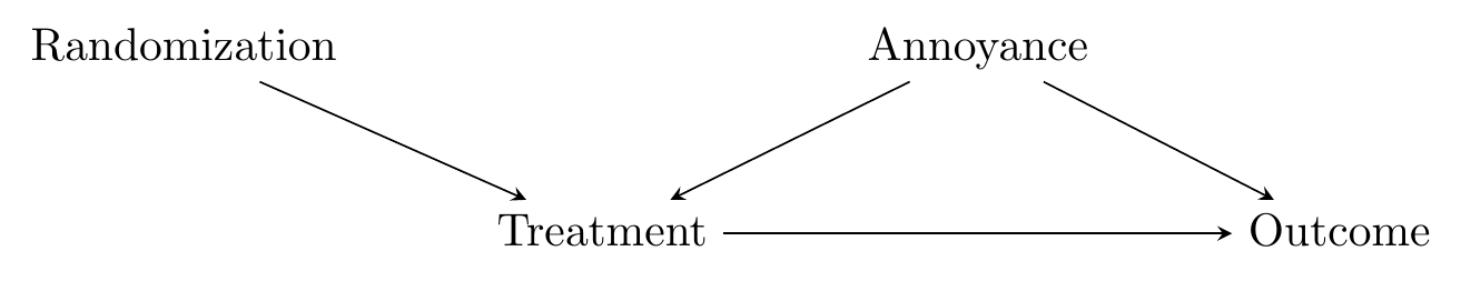
In a typical setting, if we have a \(Treatment\) and an \(Outcome\), we want to know the effect of treatment on outcome, \(Treatment \rightarrow Outcome\). However, there is, to say the least, an annoying back door path. There could be a lot going on here, but let’s just say we also have \(Treatment \leftarrow Annoyance \rightarrow Outcome\). Further, because in the social sciences \(Annoyance\) represents a bunch of different things, it’s unlikely we can control for it all. A randomized experiment shakes up this system by adding a new source of variation, \(Randomization\), that’s completely unrelated to \(Annoyance\).541 In all of this, we can refer back to the lingo from Chapter 13: \(Treatment\) is endogenous due to how it is determined by \(Annoyance\). But \(Randomization\) is exogenous, or we might say it’s “an exogenous source of variation,” because it’s not caused by anything else in the system. This is all shown in Figure 19.1.
Figure 19.1: Randomization Helps Avoid Back Doors
The instrumental variables design works in the exact same way. The only difference is that, instead of randomizing the variable ourselves, we hope that something has already randomized it for us. We look in the real world for a source of randomization that has no back doors,542 Or at least has back doors that are easily closed by controlling. and use that to mimic a randomized controlled experiment.
An instrumental variables design does not remove the requirement to identify an effect by closing back doors. But it does move the requirement, hopefully to something easier! Instead of needing to close the back doors between \(Treatment\) and \(Outcome\), which would require us to control for \(Annoyance\), we instead just need to close the back doors between \(Randomization\) and \(Outcome\) (if there are any), as well as any front door between \(Randomization\) and \(Outcome\) that doesn’t pass through \(Treatment\).
The mechanics for actually implementing instrumental variables are, in effect, a means of trying to do what an experiment does when you don’t actually have perfect control of the situation - makes sense, as that’s what is happening.
How can we mimic a randomized experiment? Well, in a randomized experiment, we generate some random variation and then just isolate the part of the treatment that is driven by that random variation - we only use the data from the experiment. So in instrumental variables we’re going to isolate just the part of the treatment that is driven by the instrument, but statistically.
In other words, we’re going to:
- Use the instrument to explain the treatment
- Remove any part of the treatment that is not explained by the instrument
- Use the instrument to explain the outcome
- Remove any part of the outcome that is not explained by the instrument543 Steps 3 and 4 here turn out to not actually make a difference for your estimate in the typical case - you end up getting the explained part of the outcome anyway if you use instrument-explained treatment to explain regular-ol’ outcome. But I keep it in because I think it makes the concept clearer.
- Look at the relationship between the remaining, instrument-explained part of the outcome and the remaining, instrument-explained part of the treatment
This is, in effect, the opposite of controlling for a variable. When we get the effect of \(X\) on \(Y\) while controlling for \(W\), we use \(W\) to explain \(X\) and \(Y\) and remove the explained parts, since we want to close any path that goes through \(W\). But when we get the effect of \(X\) on \(Y\) using \(Z\) as an instrument, we use \(Z\) to explain \(X\) and \(Y\) and remove the unexplained parts, to give us only the paths that come from \(Z\). The part that’s explained by \(Z\) is the part with no back doors, which is what we want.
The whole story can be seen in Figure 19.2, which demonstrates what an instrumental variables design actually does to data to get its estimate. The figure uses a binary instrument - this isn’t necessary for instrumental variables generally, but the figure is much easier to follow this way. We start with Figure 19.2 (a), graphing the raw data, which shows a slight positive relationship between \(X\) and \(Y\). We can also see the different values of \(Z\) on different parts of the graph - the 0s to the bottom-right and the 1s to the top-left.
We can move on to Figure 19.2 (b), which shows us taking the mean of \(X\) within the different \(Z\) values. Instrumental variables uses the part of \(X\) that is explained by \(Z\). When \(Z\) is binary, that’s just the mean of \(X\) for each group. We only want to use the part of \(X\) that’s explained by \(Z\) - that’s the part without any back doors, so in Figure 19.2 (c) we get rid of all the variation in \(X\) that isn’t explained by \(Z\), leaving us with only those predicted (mean-within-\(Z\)) \(X\) values.
Then in Figures 19.2 (d) and (e), we repeat the process with \(Y\). We do this, again, to close the back doors between \(X\) and \(Y\). That nice \(Z\)-driven variation is free of back doors, so we want to isolate just that part.
Finally, in Figure 19.2 (f), we look at the relationship between the predicted part of \(X\) and the predicted part of \(Y\). Since \(Z\) is binary, each observation in the data gets only one of two predictions - the \(Z=0\) prediction for \(X\) and \(Y\), or the \(Z=1\) prediction for \(X\) and \(Y\). Only two predictions means only two dots left on the graph, and we can get the relationship between \(X\) and \(Y\) by just drawing a line between those two points. The slope of that line is the effect of \(X\) on \(Y\), as estimated using \(Z\) as an instrumental variable, i.e., isolating only the part of the \(X\)/\(Y\) relationship that is predicted by \(Z\). The slope we have here is negative, unlike the positive relationship from (a). And since I generated this data myself, I can tell you that the true relationship between \(X\) and \(Y\) in this data is in fact negative, just like the slope in (f).
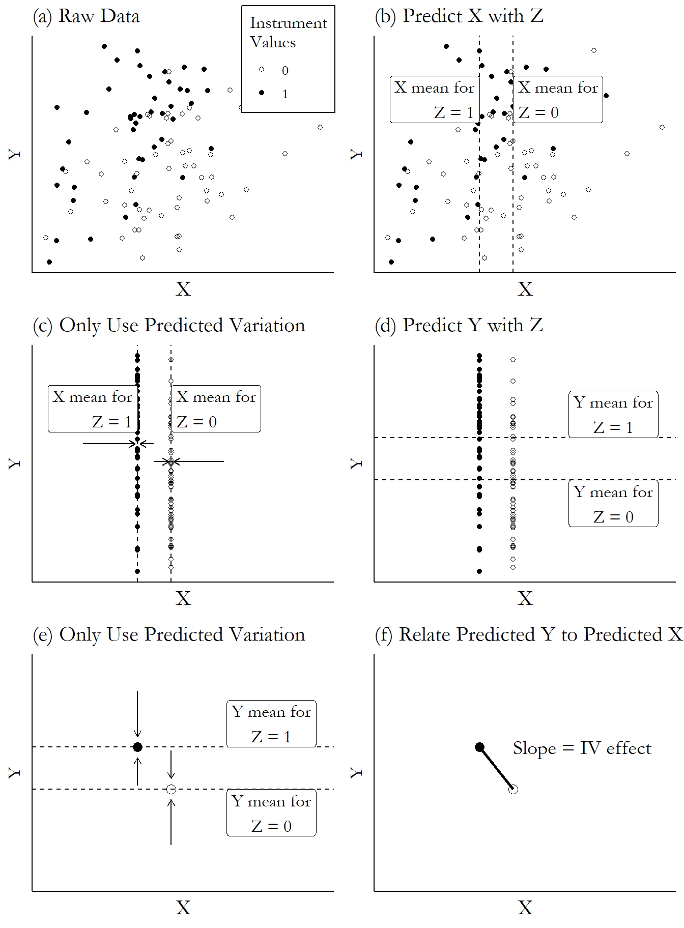
Figure 19.2: Instrumental Variables with a Binary Instrument, Step by Step
19.1.2 Assumptions for Instrumental Variables
For instrumental variables (IVs) to work, we must satisfy two assumptions: relevance of the instrument, and validity of the instrument.544 Rather, we must satisfy at least two assumptions. But these are the two with real star power that everyone talks about. Regular OLS assumptions also apply, as well as monotonicity - the assumption that the relationship between the IV and the endogenous variable is always of the same sign (or zero). We’ll talk more about monotonicity in the “How Is It Performed?” section.
Relevance is fairly straightforward. The idea of instrumental variables is that we use the part of \(X\), the treatment, that is explained by \(Z\), the instrument. But what if no part of \(X\) is explained by \(Z\)? What if they’re completely unrelated? In that case, instrumental variables doesn’t work.
This follows pretty intuitively - we can’t isolate the part of \(X\) explained by \(Z\) if there isn’t a \(Z\)-explained part of \(X\) to isolate. Also, if we follow the steps described earlier in the chapter,545 And are using a standard linear one-treatment one-instrument version of IV. then instrumental variables in effect asks “for each \(Z\)-explained movement in \(X\), how much \(Z\)-explained movement in \(Y\) was there?” In other words, in its basic form instrumental variables gives us \(Cov(Z,Y)/Cov(Z,X)\).546 Referring back to Figure 19.2 above, this is the slope you get after isolating the \(Z\)-explained parts of both variables. After all, slope is rise (how much \(Y\) increases for an increase in \(Z\)) over run (how much \(X\) increases for a given increase in \(Z\)), which is another way of thinking about a slope. If \(Z\) doesn’t explain \(X\), then \(Cov(Z,X) = 0\) and we get \(Cov(Z,Y)/0\). And we can’t divide by 0.547 Unlike starting a sentence with a conjunction, which we totally can do. The estimation simply wouldn’t work.
Now in real-world settings, hardly any correlation is truly zero. But even if \(Cov(Z,X)\) is just small rather than zero, we still have problems. If the covariance \(Cov(Z,X)\) is small, we’d call \(Z\) a weak instrument for \(X\). The estimate of \(Cov(Z,X)\) is likely to jump around a bit from sample to sample - that’s the nature of sampling variation. If \(Cov(Z,X)\) is, for example, on average 1, and it varies a bit from sample to sample, we might get values from .95 to 1.05, changing our \(Cov(Z,Y)/Cov(Z,X)\) instrumental variables estimate by maybe 10% across samples. But if \(Cov(Z,X)\) follows the same range for a much lower baseline, maybe from .01 to .11, that changes our \(Cov(Z,Y)/Cov(Z,X)\) estimate by as much as 1100% across samples. Big, swingy estimates! Big and swingy may be positive qualities in some areas of life but not in statistics.
So we need to be sure that \(Z\) actually relates to \(X\). Thankfully, this is one of the few assumptions in this half of the book we can really confidently check. Simply look at the relationship between \(X\) and \(Z\) and see how strong it is. The stronger it is, the more confident you can be in the relevance assumption, and the less the estimate will jump around from sample to sample.548 How strong does it need to be? Good question. We’ll talk about it in the next section.
Perhaps the more fraught of the two assumptions is the assumption of validity. Validity is, in effect, the assumption that the instrument \(Z\) is a variable that has no open back doors of its own.549 Validity is sometimes also called an “exclusion restriction,” because it is an assumption that \(Z\) can reasonably be excluded from the model of \(Y\) after the \(Z\rightarrow X\) path is included.
Perhaps a bit more precisely, any paths between the instrument \(Z\) and the outcome \(Y\) must either pass through the treatment \(X\) or be closed. Remember, instrumental variables doesn’t relieve us of the duty of closing all the back doors that are there; it just moves that responsibility from the treatment to the instrument, and hopefully the instrument is easier to close back doors for.
Take Figure 19.3 for example. If we want to use \(Z\) as an instrumental variable to identify the effect of \(X\) on \(Y\), what needs to be true for the validity assumption to hold?
Figure 19.3: A Diagram Amenable to Instrumental Variables Estimation… If We Pick Controls Carefully!
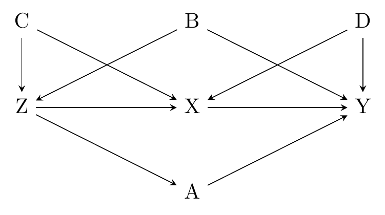
There are a few paths from \(Z\) to \(Y\) we need to think about:
- \(Z \rightarrow X \rightarrow Y\)
- \(Z \rightarrow X \leftarrow D \rightarrow Y\)
- \(Z \leftarrow C \rightarrow X \rightarrow Y\)
- \(Z \leftarrow C \rightarrow X \leftarrow D \rightarrow Y\)
- \(Z \leftarrow B \rightarrow Y\)
- \(Z \rightarrow A \rightarrow Y\)
We want all open paths from \(Z\) to \(Y\) to contain \(X\). The first four paths in the list contain \(X\), so those are good to go. It’s not even a problem that we have \(Z \leftarrow C \rightarrow X\). If that path is left open, we can’t identify \(Z \rightarrow X\). But who cares? We don’t have to identify \(Z \rightarrow X\), we just need there to be no way to get from \(Z\) to \(Y\) except through \(X\).550 We probably don’t want to control for \(C\) (although doing so wouldn’t make \(Z\) invalid). The presence of \(C\) probably strengthens the predictive effect of \(Z\) on \(X\), depending on whether those arrows are positive or negative. So controlling for \(C\) might make \(Z\) less relevant. That’s a shocker - our identification of \(X\rightarrow Y\) is actually helped in this instance by failing to identify \(Z\rightarrow X\). \(^,\)551 \(C\) would also be a great instrument in its own right on this diagram.
How about \(D\)? That’s the annoying source of endogeneity that we presumably couldn’t control for that made \(X \rightarrow Y\) unidentified and required us to use IV in the first place. But even though we have \(Z \rightarrow X \leftarrow D \rightarrow Y\), that’s fine. Once we isolate the variation in \(X\) driven by \(Z\), any other arrow leading to \(X\) basically doesn’t matter anymore. Those arrows might go to \(X\), but they don’t go to \(Z\), and we’re only using variation that starts with \(Z\).
Putting the paths with \(X\) in them to the side, that leaves us with two: \(Z \leftarrow B \rightarrow Y\) and \(Z \rightarrow A \rightarrow Y\). These two paths are problems and must be shut down for \(Z\) to be valid. \(Z \leftarrow B \rightarrow Y\) is an obvious one. That looks just like any normal back door we’d be concerned about.
But why is \(Z \rightarrow A \rightarrow Y\) a problem, too? Because it gives \(Z\) another way to be related to \(Y\) other than through \(X\). When we isolate the variation in \(X\) driven by \(Z\), that variation will also be closely related to \(A\).552 In fact, as long as we’re talking about linear models, the variation in \(X\) driven by \(Z\) will be perfectly correlated with the variation in \(A\) driven by \(Z\). So when we then look at the relationship between \(Y\) and the variation in \(X\) driven by \(Z\), we’ll mix together the effect of \(X\) and the effect of \(A\).
So for the validity assumption to hold for \(Z\), we need to close both the \(Z \leftarrow B \rightarrow Y\) path and the \(Z \rightarrow A \rightarrow Y\) path. If we can control for both \(A\) and \(B\), then we’re fine.553 Because we need to control for things to get validity to hold in this instance, we’d say that validity holds conditional on \(A\) and \(B\).
We need relevance and validity. How realistic is validity, anyway? We ideally want our instrument to behave just like randomization in an experiment. But in the real world, how likely is that to actually happen? Or, if it’s an IV that requires control variables to be valid, how confident can we be that the controls really do everything we need them to?
In the long-ago times, researchers were happy to use instruments without thinking too hard about validity. If you go back to the 1970s or 1980s, you can find people using things like parental education as an instrument for your own (surely your parents’ education can’t possibly affect your outcomes except through your own education!). It was the Wild West out there…
But these days, go to any seminar where an instrumental variables paper is presented and you’ll hear no end of worries and arguments about whether the instrument is valid. And as time goes on, it seems like people have gotten more and more difficult to convince when it comes to validity.554 This focus on validity is good, but sometimes comes at the expense of thinking about other IV considerations, like monotonicity (we’ll get there) or even basic stuff like how good the data is.
There’s good reason to be concerned. Not only is it hard to justify that there exists a variable strongly related to treatment that somehow isn’t at all related to all the sources of hard-to-control-for back doors that the treatment had in the first place, we also have plenty of history of instruments that we thought sounded pretty good that turned out not to work so well.
To pick two examples of many, we can first look at Acemoglu and Johnson (2007Acemoglu, Daron, and Simon Johnson. 2007. “Disease and Development: The Effect of Life Expectancy on Economic Growth.” Journal of Political Economy 115 (6): 925–85.). In this study, they want to understand the effect that a population’s health has on economic growth in that country. We’d expect that a healthier population leads to better economic growth, right? They use the timing of when new medical technology (like vaccines for certain diseases) is introduced as an instrument for a country’s health (specifically, mortality from certain diseases). They find that changes in health in a given year driven by changes in medical technology that year actually have a negative effect on a country’s economic growth!
Bloom, Canning, and Fink (2014Bloom, David E., David Canning, and Günther Fink. 2014. “Disease and Development Revisited.” Journal of Political Economy 122 (6): 1355–66.) have a different view on the instrument that Acemoglu and Johnson used. Bloom, Canning, and Fink point out that the original study didn’t account for the possibility that changes in health may have long-term effects on growth. Why might this matter? Because the healthier you already are, the less a new medical technology can improve your mortality rates even further. So the effectiveness of that medical technology is related to preexisting health, which is related to preexisting economic factors, which is related to current economic growth. A back door emerges. Bloom, Canning, and Fink find that when they add a control for preexisting factors, presumably fixing the validity issue, the negative effect that Acemoglu and Johnson found actually becomes positive.555 On a personal level I basically never believe the validity assumption when the data is on the level of a whole country - closing all the necessary back doors seems impossible for something so big and interconnected! “Another macro IV paper?” I chuckle and roll my eyes, tutting at the world. The fools! Then they get thousands of cites and probably a Nobel or something while I sit alone at 3 AM in the dark wondering if anyone would really notice if I submitted to a predatory pay-to-publish journal.
A particularly well-known example of a popular IV falling into disrepute is rainfall, which was a commonly-used instrument in studies of modern agricultural societies.556 These days, saying you’re going to use rainfall as an instrument is a sort of almost-funny in-joke among a certain set of causal inference nerds. The joke is completely incomprehensible to all normal people, just like the things causal inference nerds say that aren’t jokes. Rainfall levels have been used as an instrument for all sorts of things, like personal income or economic activity.557 In general, the same instrument being used as an instrument for multiple different treatments should be a cause for suspicion. After all, this implies that your instrument causes multiple things that also cause your outcome. So to get rid of all paths that don’t go through your treatment, you’re going to have to control for all the other treatments your instrument affects. This is often not possible. Less rain (or too much rain) can harm agricultural output. If everyone’s a farmer, well… that’s no good! Since farmers don’t have any control over rainfall, it seems reasonable to treat it as exogenous and without any back doors.
To follow one example of a study that uses rainfall as an instrument, Miguel, Satyanath, and Sergenti (2004Miguel, Edward, Shanker Satyanath, and Ernest Sergenti. 2004. “Economic Shocks and Civil Conflict: An Instrumental Variables Approach.” Journal of Political Economy 112 (4): 725–53.) use rainfall as an instrument for economic growth in different countries in Africa, and then look at how economic growth affects civil conflict. They find a pretty big effect: a negative change in income growth of five percentage points raises the chances of civil war by 50% in the following year.
But is rainfall a valid instrument for income? Sarsons (2015Sarsons, Heather. 2015. “Rainfall and Conflict: A Cautionary Tale.” Journal of Development Economics 115: 62–72.) looks at data from India and finds that the relationship between rainfall and conflict is similar in areas irrigated by dam water (where rainfall doesn’t affect income much) and in areas without dams (where rainfall matters for income a lot). This implies that rainfall must be affecting conflict via some mechanism other than income.558 Other authors have other reasons for doubting the validity of rainfall; this is only one of them. Sarsons lists a few other studies in her paper if you’re interested. Some of her potential explanations include rainfall spurring migration, rainfall affecting dam-fed areas by spillovers from nearby non-dam-fed areas, or rainfall making it difficult to riot or protest.
If validity is so difficult, why bother? You can’t use data to prove that your instrument is valid, and convincing others it’s valid on the basis that you think your causal diagram is right is difficult. That said, that doesn’t mean we need to give up on instrumental variables entirely. We just may need to be choosy in when we apply it.
First, there really are some situations where the instrument is as-good-as-random. You just have to pay attention and get lucky to find one! Some force happens to act to assign treatment that truly comes from outside the system or is applied almost completely randomly. A really good instrument usually takes one of two forms. Either it represents real randomization, like an actual randomized experiment, or something like “Mendelian randomization,” which uses the random process of combining parental genes to produce a child as an instrument.559 Even with something really random like Mendelian randomization, validity is not assured. If a given gene affects your treatment of interest but also some other variable that affects the outcome (perhaps the same gene affects height and weight, both of which affect athleticism), that’s a bad path! Alternately (and more common in the social sciences) a good instrument is probably one that you would never think to include in a model of the outcome variable, and in fact you may be surprised to find that it ever had anything to do with assigning treatment.
To pick one example of this kind of thing, I’ll toot my own horn and mention the only study I’ve ever worked on using a validity assumption (Goldhaber, Grout, and Huntington-Klein 2017Goldhaber, Dan, Cyrus Grout, and Nick Huntington-Klein. 2017. “Screen Twice, Cut Once: Assessing the Predictive Validity of Applicant Selection Tools.” Education Finance and Policy 12 (2): 197–223.).560 We ran a “selection model” in this paper rather than using instrumental variables, but this method similarly required a validity assumption. The paper was about the teacher hiring process in a school district that used a scoring system to evaluate applicants before hiring them. When we looked at the data, we realized that the evaluation scores on the different criteria were added up to produce an overall score by hand. Sometimes this adding-up was done incorrectly. Addition errors were a cause of making it to the next stage of the hiring process, and sound pretty random to me.561 Of course, maybe we missed something. Maybe evaluators were more likely to make errors if they didn’t like someone for some reason. It’s super important to think about what drives your instrument, just as you would think about what drives your treatment in a regular non-IV setting.
Second, there are some forms of IV analysis that allow for a little bit of failure of the validity assumption. So as long as you can make the validity assumption close to being true, you can get something out of it. We’ll talk about that in the “How the Pros Do It” section.
Third, there are certain settings where randomness is really more believable. For one, you can apply instrumental variables to actual randomized experiments, and in fact this is commonly done when not everybody does what you’ve randomized them to do (“imperfect compliance”).562 If you recall, we already talked about this back in Chapter 10 on Treatment Effects.
Did you randomize some people to take a new medication and others not to, but some people skipped their medication doses anyway? If you just analyze the experiment as normal, you’ll underestimate the effect of the medication, since you’ll have people who never actually took it mixed in there. This would be the “intent-to-treat” estimate, the effect of assigning people to take medication, rather than the effect of the medication itself. But if you use the random assignment as an instrument for taking the medication (treatment), you get the effect of treatment. And that random assignment sounds pretty darn valid. After all, it really was random. No alternate paths!
Another place where IV pops up with a really believable validity assumption is in application to regression discontinuity designs. We’ll get to those in Chapter 20. But for now, let’s get a little deeper into how we can actually use IV ourselves, if we do happen to believe that validity assumption.
19.1.3 Canonical Designs
The use of instrumental variables means you can find causal inference using all sorts of clever designs, and in all sorts of places that seem helplessly chock-full of back doors. “Clever” is probably the most common adjective you’ll hear for a good instrument.563 Although whether that word implies excitement about the design or an indictment of the whole idea of instruments depends on who is talking.
One downside of super clever instruments, though, is that they’re often highly context-dependent. But some instrumental variables designs seem to be both pretty plausible, apply in lots of different situations, and get used over and over again.564 These are generally pairs of instruments and treatments that get reused. If you had one instrument used over and over again for different treatments, that would imply the instrument wasn’t very good since for any one treatment, you’re likely to have some open front doors from instrument to outcome that don’t go through treatment - they go through treatments too. Some of these I’ve already discussed - charter school lotteries from Chapter 9 are an example. And of course the use of instruments in the case of random experiments with imperfect compliance. Another is - uh-oh - rainfall as an instrument for agricultural productivity. But others have weathered years of criticism a bit better than rainfall did.565 You may notice that most of these surviving designs have some element of explicit randomization to them; take that as you will.
One good example of a canonical instrumental variables design is judge assignment (Aizer and Doyle Jr 2015Aizer, Anna, and Joseph J. Doyle Jr. 2015. “Juvenile Incarceration, Human Capital, and Future Crime: Evidence from Randomly Assigned Judges.” The Quarterly Journal of Economics 130 (2): 759–803.). In many court systems, when you are about to go on trial, the process of assigning a judge to your trial is more or less random. This is important because some judges are harsher, and others are less harsh. This means that \(JudgeHarshness\) can act as an instrument for \(Punishment\). Simply estimate the harshness of each judge using their prior rulings. Then, the harshness of your judge is an instrument for your punishment. This can be used anywhere you have randomly-assigned judges and want to know the impact of harsher punishments (or even being judged guilty) on some later outcome.
Another is the use of the military draft as an instrument for military service (Angrist 1990Angrist, Joshua D. 1990. “Lifetime Earnings and the Vietnam Era Draft Lottery: Evidence from Social Security Administrative Records.” The American Economic Review, 313–36.). Military drafts are usually done semi-randomly, with the order in which people are drafted assigned in a random way. Whether you are drafted or not is a combination of where you are in the order and how many people they want to draft. So where you fall in the random draft order is a source of randomization for military service. It can also be a source of randomization for other things, like going to college, that may let you avoid the draft.566 Uh-oh. An instrument for two treatments! This one is a bit less of a concern than rainfall though, since these activities are sort of alternatives to each other. An instrument for any treatment would also be an instrument for not-getting-treatment. You could instead think of draft order as an instrument for “what you do after high school.”
Perhaps the most commonly used instrumental variables design ever is compulsory schooling as an instrument for years of education (Angrist and Keueger 1991Angrist, Joshua D., and Alan B. Keueger. 1991. “Does Compulsory School Attendance Affect Schooling and Earnings?” The Quarterly Journal of Economics 106 (4): 979–1014.).567 Boy, that Angrist guy gets around, huh? There are a zillion things that go into your decision of how long to continue in education and when to stop. But in many places, there is a compulsory schooling age - you can’t legally drop out until a certain age. So if you’d like to drop out at fifteen, but the law keeps you in until sixteen, that’s a little nudge of extra education for you. Variation between regions in these laws over time can act as an instrument for how much education you get.
Lastly, there’s the “Bartik Shift-Share IV” (Bartik 1991Bartik, Timothy J. 1991. Who Benefits from State and Local Economic Development Policies? WE Upjohn Institute for Employment Research.). In this design, shared economy-wide trends are combined with the distribution of industries across different regions as an instrument for economic activity. In other words, if you live in Ice Cream Town, which makes a lot of ice cream, and the next town over is Popcorn Town, which makes a lot of popcorn, and over the past ten years ice cream has gotten way more popular on a national level, that’s going to be a fairly-random boon for your town. Easy! Recent work looks more closely at this design and finds a few changes in how we interpret it (Goldsmith-Pinkham, Sorkin, and Swift 2020Goldsmith-Pinkham, Paul, Isaac Sorkin, and Henry Swift. 2020. “Bartik Instruments: What, When, Why, and How.” American Economic Review 110 (8): 2586–2624.), but the design lives on.
There are plenty of other canonical designs, of course. Settling locations of an original wave of immigrants as an instrument for further immigration, the birth of twins as an instrument for the number of children, housing supply elasticity as an instrument for housing prices, natural disasters as instruments for all sorts of things… I could go on. In the course of the chapter, I’ll talk about three other canonical designs: the direction of the wind as an instrument for pollution, whether your first two children are the same sex as an instrument for having a third, and “Mendelian randomization,” which uses someone’s genetic code as an instrument for all sorts of things.
19.2 How Is It Performed?
19.2.1 Instrumental Variables Estimators
We can start with our approach to estimating instrumental variables by taking it pretty literally. Instrumental variables as a research design is all about isolating the variation in the treatment that is explained by the instrument. So let’s just, uh, do that.
Two-stage least squares (2SLS)568 Or TSLS, but that one just looks wrong if you ask me. is a method that uses two regressions to estimate an instrumental variables model. The “first stage” uses the instrument (and other controls) to predict the treatment variable. Then, you take the predicted (explained) values of the treatment variable from that first stage, and use that to predict the outcome in the second stage (along with the controls again).
Given our instrument \(Z\), treatment \(X\), outcome \(Y\), and controls \(W\), we would estimate the models:
where \(\nu\) and \(\varepsilon\) are both error terms, \(\hat{X}\) are the predicted values of \(X\), predicted using an OLS estimation of the first equation, and \(\gamma\) are regression coefficients just like \(\beta\), only given a different Greek letter to avoid confusing them with the \(\beta\)s.569 If the goal is to close the back doors associated with the parts of \(X\) not explained by \(Z\), why don’t we take the residuals instead of the predicted values, and then control for them in the second stage, alongside regular ol’ \(X\)? Well… you could! This is called the control function approach. In standard linear IV, this produces basically the same results as 2SLS. But it has some important applications for nonlinear IV, which I’ll get to later in the chapter.
The procedure is quite easy to do by hand (although I wouldn’t recommend it, for reasons I’ll get to in a moment). Simply run OLS of \(X\) on \(Z\) (lm in R, regress in Stata, sm.ols().fit() in Python with statsmodels). Then, predict \(X\) using the results of that regression (predict() in R, predict in Stata, sm.ols().fit().predict() in Python). Finally, do a regression of \(Y\) on the predicted values. Don’t forget to include any controls in both the first and second stages.
We’re not entirely done yet - if we simply do this procedure as I’ve described it, our standard errors will be wrong. So there’s a standard error adjustment to be done, changing them to account for the fact that we’ve estimated \(\hat{X}\) rather than measuring it, and therefore there’s more uncertainty in those values than OLS will pick up on.570 For this reason, you generally will want to use a software command specifically designed for IV to run IV.
But with that under our belt, we have created our own instrumental variables estimate!
What is it doing, precisely, anyway? 2SLS produces a ratio of effects, dividing the effect of \(Z\) on \(Y\) by the effect of \(Z\) on \(X\). It asks “for each movement in \(X\) we get by changing \(Z\), how much movement in \(Y\) does that lead to?” The answer to this question, since \(Z\) has no back doors, should give us the causal effect of \(X\) on \(Y\).
2SLS has some nice features - it’s easy to estimate, it’s flexible (adding more instruments to the first stage is super easy, although adding more treatment variables is less easy), and since it really just uses OLS, it’s easy to understand. These are the reasons why 2SLS is by far the most common way of implementing instrumental variables.
2SLS has some downsides too. It doesn’t perform that well in small samples, for one. While the instrument in theory has no back doors, in an actual data set the relationship between \(Z\) and the non-\(X\) parts of \(Y\) is going to be at least a little nonzero, just by random chance. The smaller the sample is, the more often this “nonzero by random chance” is going to be not just nonzero but fairly large, driving \(Z\) to not be quite valid in a given sample and giving you bias. Additionally, 2SLS doesn’t perform particularly well when the errors are heteroskedastic.571 Heteroskedasticity-robust standard errors only do an okay job fixing this.
While two-stage least squares is the most literal way of thinking about instrumental variables, it is only one estimator of many. And there’s a good case to be made that it isn’t even that great a pick among the different estimators, despite its popularity.
Here, I’ll talk a bit about the generalized method of moments (GMM) approach to estimating instrumental variables. Some other methods, each with its own strengths, will pop up throughout the chapter.
GMM is an approach to estimation that’s much broader than instrumental variables, but in this chapter at least we’re just using it for IV.572 Many good textbooks out there go into more detail. A lot of them are titled, surprisingly enough, “Generalized Method of Moments” with a few extra words tacked on. The basic idea is this: based on your assumptions and theory, construct some statistical moments (means, variances, covariances, etc.) that should have certain values.
For example, if we want to use GMM to estimate the expected value (mean, basically) of a variable \(Y\), we’d say that the difference between our sample estimation of the expected value \(\mu\) and the population expected value \(E(Y)\) should be zero. So we’d make \(\mu - E(Y) = 0\) a condition of our estimation. Replace \(E(Y)\) with its sample value \(\frac{1}{N}\sum Y\) and solve the equation to get \(\hat{\mu} = \frac{1}{N}\sum Y\). GMM will pick the \(\mu\) that makes the moment condition true on average. Or for OLS, we assume that \(X\) is unrelated to the error term \(\varepsilon\). So we use the condition that \(Cov(X,\varepsilon) = 0\). In the actual data, that works out to \(\sum Xr = 0\), where \(r\) is the residual. Do a little math and you end up back at the same estimate for \(\beta_1\) that we already had.573 How? Let’s simplify by assuming everything is mean-zero so we don’t need an intercept. Start with \(\sum Xr = 0\). Then plug in \(r = Y - \beta_1X\) to get \(\sum X(Y-\beta_1X) = \sum(XY - \beta_1X^2) = 0\). Solve for \(\beta_1\) to get \(\beta_1 = \sum(XY)/\sum(X^2)\), which is what we had before. \(^,\)574 In the case of the mean and OLS, the solution it comes to is the same as we’ve already gotten - take the mean of the sample data. But the way we got there is different.
You might be able to guess how GMM works with IV from the OLS example. We assume that \(Z\) is unrelated to the second-stage error term \(\varepsilon\). So we use the condition \(Cov(Z,\varepsilon) = 0\). Substitute in the sample-data version of the covariance and do a little math to end up with \(\beta_1 = \sum(ZY)/\sum(ZX)\), which is what we had before.
So, same answer. Big whoop, right? Except that things get a bit more interesting when we either have heteroskedasticity (which we probably do) or add more instruments.
Overidentified. An IV model with more instrumental variables than treatment/endogenous variables.
Just identified or exactly identified. An IV model with the same number of instrumental variables as treatment/endogenous variables.
GMM and 2SLS are both capable of handling heteroskedasticity. GMM does so naturally, as it doesn’t really make assumptions about the error terms in the same way that the OLS equations making up 2SLS do. But we can get there with 2SLS by simply using heteroskedasticity-robust standard errors.
But things get more interesting when the number of instruments is bigger than the number of treatment/endogenous variables you have, which is called being “overidentified.”
When your model is overidentified, 2SLS and GMM diverge.575 In overidentified cases, GMM can’t actually satisfy all of the moment conditions exactly, so it needs to pick weights for the conditions to decide which are more important. Roughly, it weights the conditions by how difficult they are to satisfy. GMM is going to be more precise, at least if there’s heteroskedasticity involved. GMM will have less sampling variation (and thus smaller standard errors) under heteroskedasticity than 2SLS, even if you add heteroskedasticity-robust standard errors. This continues to be true if you start applying clustered standard errors or corrections for autocorrelation.
Keep in mind - GMM isn’t just a different way of adjusting the standard errors. The estimates themselves will actually be different when there’s overidentification. The GMM standard errors are smaller not because we choose to claim we have more information and thus more precision, but because the method itself produces more precise estimates, and the smaller standard errors reflect that.
Let’s code up some instrumental variables. For this exercise we’ll be following along with the paper “Social Networks and the Decision to Insure” by Cai, De Janvry, and Sadoulet (2015Cai, Jing, Alain De Janvry, and Elisabeth Sadoulet. 2015. “Social Networks and the Decision to Insure.” American Economic Journal: Applied Economics 7 (2): 81–108.). The authors are looking into the decision that farmers make about whether to buy insurance against weather events. In particular, they’re interested in whether information about insurance travels through social networks.
They look at a randomized experiment in rural China, where households were randomized into two rounds of different informational sessions about insurance. The question then is: how much does what your friends learn about insurance affect your own takeup of insurance? They look at people in the second round of sessions, and they look at what their friends did and saw in the first round of sessions, to see how the former is affected by the latter.576 By structuring things in this way where they look only at the effect of the first round on the second, they avoid “reflection,” a common problem with studies about how your friends affect what you do; these studies are also known as studies of “peer effects.” The reflection problem, attributed to perennial Nobel overlookee Charles Manski, points out the identification problem you face if you want to learn about how your friends affect you… the problem being that you affect your friends too! There’s a feedback loop, and we know that a causal diagram hates a feedback loop. By having a first round and a second round, we know which direction the causal arrow points.
Cai, De Janvry, and Sadoulet do in general find that farmers’ decisions were affected by what their friends saw and the information they received. I’ll be looking at a particular one of their analyses where they ask whether farmers’ decisions were affected by what their friends did: does your friends actually buying insurance make you more likely to buy?
We want to identify the effect of \(FriendsPurchaseBehavior\) on \(YourPurchaseBehavior\) among people in the second-round informational sessions, looking at the average purchasing behavior of their friends who were in the first-round informational sessions. This effect has some obvious back doors. Preferences for insurance may be higher or lower by region, or you may simply be more likely to have friends with preferences similar to yours, including on topics like insurance.
As an instrument for \(FriendsPurchaseBehavior\) they use the variable \(FirstRoundDefault\), which is a binary indicator for whether your friends were randomly assigned to a “default buy” informational session, where attendees were assigned to buy insurance by default, and had to specify their preference not to buy it, or a “default no buy” session, where attendees were assigned to not buy insurance by default, and had to specify their preference to buy it. Everyone had the same options and got the same information, but the defaults were different. People follow defaults! Those in the “default buy” sessions were twelve percentage points more likely to buy insurance than those in the “default no buy” sessions. The fact that \(FirstRoundDefault\) is randomized makes the argument that it’s a valid instrument pretty believable. Plus, a twelve percentage point jump seems like plenty to satisfy the relevance assumption.577 We’re going to use the analysis they did on the subsample of second-round participants who were told what purchasing decisions their first-round friends had made. They did another analysis with second-round participants who were not told, and found no effect.
Okay, now, finally let’s code the thing. We’ll start with 2SLS, and then, using the same data, will do GMM, LIML, and IV with fixed effects (“panel IV”). Wait, I slipped “LIML” in there - what’s that? That’s limited-information maximum likelihood. I’ll show how to code it up here, since it’s easy enough to switch out methods, but I’ll actually talk about the method later in the chapter.
R Code
# There are many ways to run 2SLS;
# the most common is ivreg from the AER package.
# But we'll use feols from fixest for speed and ease
# of fixed-effects additions later
library(tidyverse); library(modelsummary); library(fixest)
d <- causaldata::social_insure

# Include just the outcome and controls first, then endogenous ~ instrument
# in the second part, and for this study we cluster on address
m <- feols(takeup_survey ~ male + age + agpop + ricearea_2010 +
            literacy + intensive + risk_averse + disaster_prob +
            factor(village) | pre_takeup_rate ~ default,
            cluster = ~address, data = d)

# Show the first and second stage, omitting all
# the controls for ease of visibility
msummary(list('First Stage' = m$iv_first_stage$pre_takeup_rate,
                'Second Stage' = m),
                coef_map = c(default = 'First Round Default',
                fit_pre_takeup_rate = "Friends' Purchase Behavior"),
                stars = c('*' = .1, '**' = .05, '***' = .01))
Stata Code
causaldata social_insure.dta, use clear download

* We want village fixed effects, but that's currently a string
encode village, g(villid)

* The order doesn't matter, but we need controls here
* as well as (endogenous = instrument)
* don't forget to specify the estimator 2sls!
* and we cluster on address
* and also show the first stage with the first option
ivregress 2sls takeup_survey (pre_takeup_rate = default) male age agpop ///
    ricearea_2010 literacy intensive risk_averse disaster_prob ///
    i.villid, cluster(address) first
Python Code
import pandas as pd
from linearmodels.iv import IV2SLS
from causaldata import social_insure
d = social_insure.load_pandas().data

# Add a [endogenous ~ instrument] segment to the formula
m = IV2SLS.from_formula('''takeup_survey ~
male + age + agpop + ricearea_2010 + literacy +
intensive + risk_averse + disaster_prob + C(village) +
[pre_takeup_rate ~ default]''', data = d)

# since we want to cluster, and will use
# m.notnull to see which observations to drop
second_stage = m.fit(cov_type = 'clustered',
clusters = d['address'][m.notnull])

# If we want the first stage we must do it ourselves!
# move the endogenous variable to the dependent position
# and make the instrument a predictor, removing the []
first_stage = IV2SLS.from_formula('''pre_takeup_rate ~
male + age + agpop + ricearea_2010 + literacy +
intensive + risk_averse + disaster_prob + C(village) +
default''', data = d).fit(cov_type = 'clustered',
clusters = d['address'][m.notnull])

first_stage
second_stage
This gives us the result in Table 19.1 (keeping in mind this table doesn’t show a bunch of coefficients for all the control variables).578 Copyright American Economic Association; reproduced with permission of the American Economic Journal: Applied Economics. The first stage regression has the endogenous variable (whether your friends purchased insurance) as the dependent variable, and a coefficient for our instrument. The coefficient is .118 and statistically significant. It’s showing that your friends being assigned to the “default-purchase” experimental condition leads to a 11.8 percentage point increase in the probability that they’ll buy insurance. We predict whether your friends bought insurance using that .118 bump (as well as the other predictors not shown on the table) and use those predicted values in the second stage.
| First Stage | Second Stage | |
|---|---|---|
| First Round Default | 0.118*** | |
| (0.034) | ||
| Friends Purchase Behavior | 0.791*** | |
| (0.273) | ||
| Num.Obs. | 1378 | 1378 |
| R2 | 0.469 | 0.127 |
| R2 Adj. | 0.448 | 0.092 |
| RMSE | 0.18 | 0.47 |
| Std.Errors | by: address | by: address |
| * p < 0.1, ** p < 0.05, *** p < 0.01 | ||
| Controls for gender, age, agricultural proportion, farming area, literacy, intensiveness of assigned treatment, risk aversion, perceived disaster probability, and village excluded from table. |
The second stage has the actual outcome of you buying insurance as the outcome. A one-unit increase in the rate at which your friends buy insurance, using only the random variation driven by the random experimental assignment and the controls, increases your chances of buying insurance by .791. That’s a pretty strong spillover effect!
That’s 2SLS. How about GMM and LIML? In Stata and Python the transition is easy. In Stata, run ivregress gmm or ivregress liml instead of ivregress 2sls. Unfortunately, there are some important LIML parameters \(\alpha\) and \(\kappa\) we’ll discuss later that ivregress liml won’t let you set on your own. In Python, you can use IVGMM or IVLIML instead of IV2SLS, and IVLIML does give you control over \(\alpha\) and \(\kappa\).
And in R? In R we unfortunately have to switch packages, at least for now. The ivmodel() function in the ivmodel package is capable of doing LIML, with options for setting \(\alpha\) and \(\kappa\). How about GMM? For the moment, you’ll have to set up the whole two-equation GMM model yourself using the gmm() function in the gmm package, although your options for standard error adjustments are a bit more limited. There is also the momentfit package which has some nice improvements but is similarly difficult to set up. The syntax for this example is:
R Code
library(modelsummary); library(gmm)
d <- causaldata::social_insure
# Remove all missing observations ourselves
d <- d %>%
    select(takeup_survey, male, age, agpop, ricearea_2010,
           literacy, intensive, risk_averse, disaster_prob,
           village, address, pre_takeup_rate, default) %>%
    na.omit()

m <- gmm(takeup_survey ~ male + age + agpop + ricearea_2010 +
         literacy + intensive + risk_averse + disaster_prob +
         factor(village) + pre_takeup_rate,
         ~ male + age + agpop + ricearea_2010 +
         literacy + intensive + risk_averse + disaster_prob +
         factor(village) + default, data = d)

# We can apply the address clustering most easily in msummary
msummary(m, vcov = ~address, stars = c('*' = .1, '**' = .05, '***' = .01))
Finally, what if we have a lot of fixed effects in our IV model? There are some technical adjustments that must be made in these cases. This time it’s R that has the easiest transition. The feols() function we already used can easily incorporate fixed effects - the +factor(village) just becomes | village. Stata and Python aren’t too hard though. In Stata you switch from ivregress to xtivreg. This comes with a few other changes - you must xtset your data to tell Stata what the panel structure is, it only does 2SLS rather than GMM or LIML, and you must tell it whether you want fixed effects (fe), random effects (re), or something else (see the help file). At the moment, there is no Python equivalent for this, although our typical Python syntax will let you estimate IV models with fixed effects in them by adding sets of binary indicator variables.
19.2.2 Instrumental Variables and Treatment Effects
What does instrumental variables estimate? We can refer back to Chapter 10 when thinking about what kind of treatment effect average instrumental variables produces.
In general, we know that IV is a method all about isolating the variation in treatment that is explained by the instruments. This means we are looking at a local average treatment effect, where the individual treatment effects are weighted by how responsive that individual observation is to the instrument.
In the case of a standard estimator like 2SLS or GMM with one treatment/endogneous variable and one instrument, the weights are what the individual effect of the instrument would be for you in the first stage.
For example, say there has been a recent set of television advertisements that encourage people to exercise more. You want to use exposure to the advertisements as an instrument for how much you exercise, and then you will look at the effect of exercise on blood pressure.
Consider three people in the sample: Jakeila, Kyle, and Li. The advertisements would make Jakeila exercise an additional half hour each week, and an additional hour of exercise each week would lower her blood pressure by 2 points. You can see these values, as well as the values for Kyle and Li, on Table 19.2.
Table 19.2: Effect Sizes for Three People in our Exercise Study
| Name | Effect of Ads on Exercise Hours | Effect of Exercise Hours on Blood Pressure |
|---|---|---|
| Jakeila | 0.50 | -2 |
| Kyle | 0.25 | -8 |
| Li | 0.00 | -10 |
Keep in mind - those effects of ads on exercise hours are what the effect theoretically would be for those individual people. Obviously we can’t see Jakeila both advertised to and not advertised to at the same time. But this is saying that Jakeila-with-ads exercises half an hour more each week than Jakeila-without-ads.
What will 2SLS tell us the effect of exercise hours on blood pressure is? Well, Jakeila responds the strongest to the ads, so the -2 effect of exercise that she gets will be more heavily weighted. Specifically, it gets the .5 weight she has on the effect of ads. Similarly, Kyle gets a weight of .25. Li, on the other hand, doesn’t respond to the ads at all - they make no difference to him. So it turns out he makes no difference to the 2SLS estimate. He gets a weight of 0.
When we perform our 2SLS estimation, it can’t see any of these theoretical individual-person effects. Regardless, the LATE it gives us is based on them! Specifically, the LATE is
That’s what 2SLS will give us. This is in contrast to the average treatment effect which is \(((-2) + (-8) + (-10))/3 = -6.67\).
This immediately points us to a very important result: 2SLS will give different results depending on which IV is used. If we had picked an instrument that was really effective at getting Li to exercise but not so effective for Jakeila, then 2SLS would estimate a much stronger effect of exercise on blood pressure.
What if there’s more than one instrument? The same logic applies - the stronger the effect of the instrument for you, the more strongly your treatment effect will be weighted. But at this point the math gets a bit more complex, because it’s going to be a mix of the different weights you’d have had from the different instruments. So if one instrument would give Jakeila a .5 weight, but a different one would give her .8, the weight she’d get from using both instruments would be some mix of the .5 and .8 (and not necessarily just an average of the two).
One thing to emphasize here is that the specific weights we get are dependent on the estimator. Different ways of estimating instrumental variables can produce different weighted average treatment effects. If you’re not using 2SLS, do look into what precisely you are getting. Although outside of some corner cases you are generally still getting something that weights you more strongly the more you are affected by the instrument. The idea that we’re estimating a LATE does hold up in most cases, although the specifics on which LATE we’re getting change from estimator to estimator.
There’s a common terminology used in instrumental variables when thinking about these weights, and in particular the 0s. We can divide the sample into three groups:
- Compliers: For compliers, the effect of the instrument on the treatment is in the expected direction. Jakeila and Kyle were compliers in Table 19.2 because the ad telling them to exercise more got them to exercise more.
- Always-takers/never-takers: Always-takers/never-takers are completely unaffected by the instrument. Li was an always-taker/never-taker in Table 19.2 because the effect of the ads on his exercise level was zero.579 The terminology here comes from cases where the treatment variable is binary. “Always-takers” always get the treatment, regardless of the instrument, and “never-takers” never get the treatment, regardless of the instrument. The terms are a little odd applied to continuous treatments like we have here in exercise, but it’s the same idea.
- Defiers: Defiers are affected by the instrument in the opposite of the expected direction.580 If there are people affected in both directions in the sample, it’s a bit arbitrary to call one of them “compliers” and the other “defiers,” but the important thing really is that there are people in both directions.
From this terminology we can get one result and one assumption we need to make:
First, the result: if all of the compliers are affected by the instrument to the same degree, then 2SLS gives the average treatment effect… among compliers.581 You will find no shortage of people telling you that the LATE is the same thing as the average treatment effect among compliers. But that’s not really true, and relies on this assumption that the instrument is equally effective on all compliers. Neat! Although it is unlikely that everyone is affected in the same way by the instrument.
Second, the assumption: for all of this to work, we need to assume that there are no defiers. Imagine we add a fourth person to Table 19.2: Macy, who is so annoyed by the ads that she decides to exercise .25 hours less if she sees them. An hour of weekly exercise would reduce her blood pressure by 8 points.
How do the LATE weights work out now? Macy gets a weight of -.25. The weighted-average calculation now gives us
Exercise was actually more effective for Macy than the effect we already estimated, but adding her made the effect shrink! This is because she had a negative weight, which makes the math of weighted averages get all wonky so they’re not really weighted averages any more.582 Importantly, the problem here isn’t that Macy is affected negatively, it’s that she’s affected in a different direction to the others. Conformity is pretty helpful here. It wouldn’t be a problem if everyone had a negative effect. Then, all the negatives on the weights would just factor out. It’s like multiplying the original LATE calculation by \(-1/-1 = 1\). Makes no difference.
Monotonicity. In the context of instrumental variables, the assumption that for everyone in the data, the instrument either affects them in the same direction (positively or negatively), or not at all (zero effect).
The assumption that there are no defiers is also known as the monotonicity assumption. Along with validity and relevance, this is another key assumption we need to make for instrumental variables, although this one tends to receive a lot less attention.
So if you have an instrument that has an effect on average, think carefully about whether that effect is likely to be in the same direction for everyone. There are plenty of cases where it wouldn’t be, for example, if there are people out there who would be so annoyed by an intervention that it would have the opposite effect of what’s intended.
Or, more broadly, people are just different and react in different ways. Angrist and Evans (1998Angrist, Joshua D., and William N. Evans. 1998. “Children and Their Parents’ Labor Supply: Evidence from Exogenous Variation in Family Size.” American Economic Review 88 (3): 450–77.) are a good example for thinking about this. They observed that families appeared to have a preference for having both a boy and a girl. A family that happens to have two boys as their first two children, or two girls, would be more likely to have a third child so as to try for a mix. So, “your first two kids being the same gender” has been used as an instrument for “having a third child” in a whole bunch of studies, following on from Angrist and Evans.
But for this to work, there have to be no defiers. Even if most people would be more likely to have the third kid if the first two are the same gender (or not base their third-kid decision on that at all), if there are some people who would be less likely to have the third kid because the first two are the same gender, then monotonicity is violated. Maybe some parents are terrified by the possibility of three kids of the same gender? Whatever story we come up with, people have a lot of complex reasons for choosing to have more kids, and some of them might contradict what we need them to be. So studies using this instrument need to think carefully about whether monotonicity is likely to be satisfied, and what they can do about it.
19.2.3 Checking the Instrumental Variables Assumptions
For IV to do what we want it to, we are relying on the relevance assumption. Remember, the relevance assumption is the assumption that the instrumental variable \(Z\) and the treatment/endogenous variable \(X\) are related to each other.
We can go a bit further and say that we need to assume that \(X\) and \(Z\) are strongly enough related to each other that we don’t run into the “weak instruments problem.”
Weak instrument. An instrument that only weakly predicts the treatment/endogenous variable(s).
A weak instrument is one that is valid and does predict the treatment variable, but it only predicts the treatment variable a little bit. It predicts weakly. Keeping in mind our general intuition that IV gives us \(Cov(Z,Y)/Cov(Z,X)\), then if \(Cov(Z,X)\) is small, we’re nearing a divide-by-zero problem! The estimate as a whole balloons up really big (since you’re dividing by something tiny) and the sampling variation gets huge.
Thankfully, unlike a lot of the assumptions we cover, weak instruments (and by extension relevance) is fairly easy to test for.583 Although maybe it’s not the best way to deal with the weak-instrument problem… read to the end of the section. After all, we just need to make sure that \(Z\) and \(X\) are related, and not in a weak way. We know how to measure and test relationships!
By far the most common way to check for relevance is the first-stage F-statistic test.584 This is sometimes referred to as an underidentification test. Conveniently, it’s also the easiest. All you have to do is:
- Estimate the first stage of the model (regress the treatment/endogenous variable on the controls and instruments)
- Do a joint F-test on the instruments
- Get the F-statistic from that joint F-test and use it to decide if the instrument is relevant
That’s it! The calculation gets a bit trickier if there’s more than one treatment/endogenous variable (since there’s not really a single first stage in the same way), but the idea remains the same.
We covered the code for doing a joint F-test back in Chapter 13 on Regression, but because this is such a common test, your IV command will often do it for you. In R, if your feols regression is stored as m, summary(m) will report a “first-stage F-statistic.”585 If you’re using a different IV command, this may not work. Many of them, such as ivreg from the AER package, work with summary(m, diagnostics = TRUE). In Stata you can follow your ivregress command with estat firststage.586 If you’ve done 2SLS, this will also give you the different relevant critical values, which we’ll discuss in a second. In Python with statsmodels you can do IV2SLS().fit().first_stage and look at the “partial F-stat.”
We’ve got our first-stage F-statistic now. How big does it need to be? Checking if the instrument is statistically significant is not nearly enough - we aren’t just concerned that the relationship is zero, we’re concerned that it’s small.
Since there’s no single precise definition of “small,” there’s no single correct cutoff F-statistic to look for. Instead, we have a tradeoff. The bigger your F-statistic, the less bias you get. So the F-statistic you want will be based on how much bias you’re willing to accept.
Wait - what bias? Who said anything about bias? Weak instruments lead to bias because, even if the instrument is truly valid, in an actual sample of data the instrument will have a nonzero relationship with the error term just by random chance, worsening validity and giving you bias. The weaker the instrument is, the worse this gets.
We can frame our choice of cutoff F-statistic in responding to this tradeoff. Stock and Yogo (2005Stock, James H., and Motohiro Yogo. 2005. “Testing for Weak Instruments in Linear IV Regression.” In Identification and Inference for Econometric Models: Essays in Honor of Thomas Rothenberg, 80–108. Cambridge: Cambridge University Press.) calculate the bias that you get with instrumental variables relative to the bias you’d get by just running OLS on its own. The stronger the instrument is, the less the IV bias will be relative to the OLS bias. For especially weak instruments, you may as well just go back to OLS (or, if that doesn’t work either, you may be out of luck). Their tables at the end of the paper will show you that, for example, if you have one treatment/endogenous variable and three instruments, you need an F-statistic above 13.91 to reduce IV bias to less than 5% of OLS bias in 2SLS, but only an F-statistic above 9.08 to reduce IV bias to less than 10% of OLS bias. What if you have four instruments? Then you need 16.85 or 10.27. Some first-stage test commands (like Stata’s) will tell you the relevant cutoffs automatically.587 There is another rule of thumb that just says your F-statistic must be 10 or above in general. That’s certainly much easier to remember than looking up a value in a table, but it’s also very rough. Like many one-size-fits-all values in statistics, this is a tradition probably better left behind.
What to do if your F-statistic doesn’t measure up? You could just give up at that point - more than a few researchers would advise ditching a project with a small first-stage F-statistic. But this practice is bad if everyone does it, especially if you’re talking about projects that might end up getting published. If low-F-statistic projects get dropped based on an F-statistic cutoff, then the projects that do get published will be a mix of actually-strong IVs and actually-weak IVs where the researcher just happened to get a sample where the F-statistic was large. When an actually-weak IV happens to produce a large F-statistic, that’s what gives us the exact kind of weak-instrument bias we were worried about. We’re specifically selecting projects to complete based on getting samples where the instrument is invalid by random chance. So the F-statistic cutoff leads to a larger proportion of biased results in the published literature.
What to do? In the case of weak instruments, as long as you are indeed pretty certain that the instrument is valid, instead of ditching the project, you might want to try an approach to IV that is more robust to weak instruments. A few of these methods, like Anderson-Rubin confidence intervals, are shown in the “How the Pros Do It” section.
In fact, you may just want to go ahead and use those weak-instrument-robust methods from “How the Pros Do It” anyway. The problem with weak instruments is that they introduce a lot of sampling variation and mess with your standard errors. The idea with pre-testing is that you only pursue analyses where you know the problem isn’t too big. But that doesn’t mean the problem goes away. Lee et al. (2022Lee, David S., Justin McCrary, Marcelo J Moreira, and Jack Porter. 2022. “Valid t-Ratio Inference for IV.” American Economic Review 112 (10): 3260–90.) show that your confidence intervals will at least be a teeny bit wrong all the way up to a first-stage \(F\) statistic of 104.7. Keane and Neal (2022Keane, Michael P., and Timothy Neal. 2022. “A Practical Guide to Weak Instruments.” Annual Review of Economics 16.) show that typical cutoffs ignore things like statistical power, and there are very realistic scenarios where you’d want at least 50. Yikes! That doesn’t mean toss out anything with \(F\) below 104.7 or 50 or anything like that. Instead it just means that maybe pre-testing isn’t going to solve the real problem.
So we can test for relevance and weak instruments. How about validity? There are a few tests I should probably mention, despite the fact that they make me grumpy. In particular, there are several very well-known tests that are designed to test the validity assumption. While these tests have their uses, they are commonly applied in a way that I find thoroughly unconvincing, for reasons I’ll mention. However, they are very common and so worth at least knowing enough about to know what’s going on.
First off, what does it mean exactly to test for validity? We want to test whether there are any open back doors between the instrument \(Z\) and the outcome \(Y\). We can reframe this as checking whether \(Z\) is related to the second-stage error term \(\varepsilon\). We want \(Z\) and \(\varepsilon\) to be unrelated. If they’re related, validity is violated.
Testing for validity has some obvious hurdles to overcome. First off, we can’t actually observe the error term \(\varepsilon\), and so can’t just look at the relationship between \(Z\) and \(\varepsilon\).
Why not just look at the relationship between \(Z\) and the residual \(r\) instead? We use \(r\) in place of \(\varepsilon\) all the time for calculating things like standard errors. However, if \(Z\) is invalid, then the second-stage estimates will be biased, which will make the residuals not a great representation of the error. Since the error is the difference between the true-model prediction and the outcome, and we know that the model is biased, the estimated model isn’t even the true model on average, so the residuals don’t represent the errors very well.
What, then, can we do?
One approach that you see a lot, but that actually doesn’t make any sense, is to run the second-stage model but include the instrument as a control.
If the coefficient on the instrument \(Z\) is nonzero, that suggests a violation of validity. Why? Because all open paths from \(Z\) to \(Y\) should run through \(X\), right? So if we look at the effect of \(Z\) on \(Y\) while controlling for \(X\), that should close all pathways. If there’s still a relationship evident in \(\hat{\beta}_2\), then it seems that there are other, validity-breaking pathways still open! I keep saying it suggests'' andseems like’’ that because it doesn’t actually tell you anything! Why not? Collider bias! If both \(Z\) and \(\varepsilon\) cause \(X\), then even if \(Z\) and \(\varepsilon\) are unrelated, they’re suddenly related again if you control for \(X\), which we’re doing here. So we get a biased estimate of \(\beta_2\), and that estimate doesn’t tell us anything about the direct effect of \(Z\) on \(Y\).
Another approach uses the Durbin-Wu-Hausman test. The Durbin-Wu-Hausman test compares the results from two models, one of which may have inconsistent results if some assumptions are wrong, while the other doesn’t rely on those assumptions but is less precise. If the results are similar, it suggests that the assumptions at least aren’t so wrong that they mess up the results, and it means a green light to use the more precise model.
In the context of instrumental variables, Durbin-Wu-Hausman is used in two ways. First, it can be used to compare OLS (inconsistent if \(X\) is related to \(\varepsilon\)) to IV (less precise). If the results are different, that means that \(X\) really does have open back doors, and we should probably be using IV.
Second, Durbin-Wu-Hausman can be used to compare two different IV models in an overidentification test. If we have more instruments than we need (we are overidentified), then as long as we’re really certain that we have as many valid instruments as we need, we can compare the IV model that uses all of our instruments (inconsistent if some of them are invalid) against an IV model that only uses the instruments we’re really sure about (less precise). If they’re different, that tells us that the additional instruments are likely invalid.
In practice, overidentification tests are more commonly performed for 2SLS using a Sargan test, which gets the residuals from the second stage of a 2SLS model and looks at the relationship between those residuals and the instruments. For GMM models, often a Hansen test is used, which I won’t go into deeply here. For all of these tests, there are many ways to go at them.
In R you get both Durbin-Wu-Hausman exogeneity tests and Sargan overidentification tests automatically when you summary() the IV model you get from feols. If you’re using a different command, you may need to use the diagnostics = TRUE option. In Stata you can follow your regression with estat endog to test OLS vs IV or estat overid to do the Sargan test. In Python you can get the Durbin-Wu-Hausman exogeneity test from your model with the .wu_hausman() method, or the Sargan test with .sargan().
So those are the main tools in our belt for testing for validity of instruments. Why do they make me grumpy? Because people try to use them to justify iffy instruments. Imagine someone was showing you some research with an instrument that you didn’t think was valid, or an OLS model with a treatment you thought had some open back doors remaining. But ah - no worries! They’ve done an endogeneity test and have failed to reject the null hypothesis that the iffy treatment/instrument is valid. No problem, right?
Still a problem! There’s a lot that goes into whether a null hypothesis is rejected other than whether the underlying thing you’re testing is true or not - statistical power, sampling variation, and so on. Failing to find evidence of a validity violation could mean the instrument is valid, or it could mean one of those other things.
A more reasonable use of these tests is when you have an instrument that you are really certain about, but are worried that maybe you’ve just had a bad luck of the draw. Using these tests to disappoint yourself about an instrument you were pretty certain on is a much more justifiable use of them than using them to reassure yourself about an instrument you’re uncertain on.588 Good ol’ statistics, always looking for a way to disappoint.
There’s another reason these tests, in particular overidentification tests, make me grumpy. It has to do with the local average treatment effect (LATE) estimate being produced by the instrumental variables model. When you have more than one instrument, those instruments will generate different LATE estimates, because they explain different parts of variation in the treatment. When you combine the two instruments, you’ll get yet again another LATE.589 For more specific details on how exactly they’re combined, see Mogstad, Torgovitsky, and Walters (2021Mogstad, Magne, Alexander Torgovitsky, and Christopher R. Walters. 2021. “The Causal Interpretation of Two-Stage Least Squares with Multiple Instrumental Variables.” American Economic Review 111 (11): 3663–98.), which also shows that monotonicity needs to hold for each of your instruments while holding the other instruments constant for this to work. So if your overidentification test finds that the model produces different results with different instruments, well… that doesn’t necessarily mean that the instruments are invalid. It just means that the instruments don’t produce the same results (Parente and Silva 2012Parente, Paulo M. D. C., and J. M. C. Santos Silva. 2012. “A Cautionary Note on Tests of Overidentifying Restrictions.” Economics Letters 115 (2): 314–17.).
19.3 How the Pros Do It
19.3.1 Don’t Just TEST for Weakness, Fix It!
Weak instruments are a real problem. I’ve already discussed ways to try to detect weak instruments using an F-test. But this test has its own problems. We could, instead, just go ahead and use a method for estimating instrumental variables that is not as strongly affected by weak instruments. They do exist!
The first fix is also the easiest. In the case where we have one treatment/endogenous variable and one instrument,590 Let’s be honest, this is by far the most common scenario. Why did we bother with those overidentification tests again? we can adjust the standard errors to account for the possibility that the instruments are weak.
This solution is very old, as far back as 1949. Anderson-Rubin confidence intervals provide valid measures of uncertainty in our estimate of the effect even if the instruments are weak (Anderson and Rubin 1949Anderson, Theodore W., and Herman Rubin. 1949. “Estimation of the Parameters of a Single Equation in a Complete System of Stochastic Equations.” The Annals of Mathematical Statistics 20 (1): 46–63.).591 This is not to be confused with the Anderson-Rubin test of weak instruments. Confusing, I know. This doesn’t really solve the problem of having a weak instrument. That is, you still have a weak instrument and have the sampling variation issues that go along with it. But it does make sure that your results reflect that variation. In other words, they’ll be more honest about your weak-instrument problems.
That’s… that’s really it. If you have one instrument and one treatment/endogenous variable, you may as well skip the whole process of testing for weak instruments and just report Anderson-Rubin confidence intervals whether your instrument is weak or not. It’s kind of a shocker that this isn’t a completely universal practice. As you’ll see in the next paragraph, it isn’t even included as an option in common IV commands. We’ve known about it for ages. Ah, well.
In R you can get Anderson-Rubin confidence intervals by first estimating your IV model using the ivreg function in the AER package, and then passing that to the anderson.rubin.ci function in the ivpack package. In Stata you can get Anderson-Rubin confidence intervals by following up your ivregress model with the weakiv function from the weakiv package. To my knowledge, there’s no prepackaged way of getting Anderson-Rubin confidence intervals in Python.
A newer method, “valid t-ratio inference,” comes from Lee et al. (2022Lee, David S., Justin McCrary, Marcelo J Moreira, and Jack Porter. 2022. “Valid t-Ratio Inference for IV.” American Economic Review 112 (10): 3260–90.). This method sticks to more standard types of 2SLS statistics, but adjusts the standard errors and confidence intervals to account for the additional noise the first-stage estimation and weak instruments can lead to. Valid t-ratio inference can be performed in R in the ivDiag package. In Stata the tf package can be installed using net install tf, force from(http://www.princeton.edu/~davidlee/wp/).
We can more honestly report our weak-instrument problem, but can we really fix it? Maybe!
A common estimation method that attempts to perform better when the instrument is weak is limited-information maximum likelihood (LIML).592 Limited-information maximum likelihood is often supported by the same IV estimation software that supports 2SLS and GMM, and the code for estimation using LIML was discussed earlier in this chapter.
In short, instrumental variables uses the parts of the treatment/endogenous variable \(X\) and the outcome \(Y\) that are predicted by the instrument \(Z\). LIML in the context of instrumental variables does the same thing, except that it scales down the prediction, making it weaker, using a parameter \(\kappa\), which is generally estimated in the model based on the data. If \(\kappa=1\), we scale the prediction by 1, making no change, and ending up back with 2SLS. But if \(\kappa<1\), we bring back a little of the original endogenous variable we would have used in OLS, relying less on that weak instrument.
We can also make adjustments to \(\kappa\) using the parameter known as Fuller’s \(\alpha\). Instead of \(\kappa = \hat{\kappa}\) estimated on the basis of the data, \(\alpha\) makes it even smaller, using instead \(\kappa = \hat{\kappa} - \alpha/(N-N_I)\), where \(N\) is the number of observations and \(N_I\) is the number of instruments. \(\alpha = 4\), for example, minimizes the mean squared error of the estimate across samples. It can also be estimated using the data. The LIML procedure reduces the bias that comes along with weak instruments, but this may come, surprise surprise, at the expense of worse precision (Blomquist and Dahlberg 1999Blomquist, Sören, and Matz Dahlberg. 1999. “Small Sample Properties of LIML and Jackknife IV Estimators: Experiments with Weak Instruments.” Journal of Applied Econometrics 14 (1): 69–88.).
Anything else? One of the most promising avenues of research looks at the use of lots of weak instruments. Sure, no one of them means much for the treatment. But an army of them? This is the finale to a movie. I cannot possibly do the whole literature justice here, but one starting place is with Chao and Swanson (2005Chao, John C., and Norman R. Swanson. 2005. “Consistent Estimation with a Large Number of Weak Instruments.” Econometrica 73 (5): 1673–92.).
19.3.2 Way Past LATE
Are we stuck with local average treatment effects? Not at all! A local average treatment effect is what 2SLS gives us by default, but there are other approaches. There’s a wide literature out there on various approaches to instrumental variables estimation that produce average treatment effects (or other averages) instead of a local average treatment effect. Naturally, they all rely on different assumptions or apply in different contexts.
I’ll mention only two here, briefly. These are only two papers representing two different general approaches to getting average treatment effects, and those two approaches are far from the only two.593 And a third, in fact, will pop up in the next section. These are starting points.
First, Heckman and Vytlacil (1999Heckman, James J., and Edward J. Vytlacil. 1999. “Local Instrumental Variables and Latent Variable Models for Identifying and Bounding Treatment Effects.” Proceedings of the National Academy of Sciences 96 (8): 4730–34.) look at instrumental variables that take lots of different values. They realize that you can identify a bunch of effects by comparing different values—what’s the treatment effect among those pushed from the very lowest value of the instrument to just above that? What’s the effect from those pushed from the just-above-that value to just-above-that? And so on. So now you’ve got a whole bunch of effects for the range of the instrument. Under the condition that the probability of treatment is zero for some values of the instrument, and one for others, you can average out this whole distribution of effects to get an average treatment effect.
Second is the literature using correlated random effects (remember those from Chapter 16?) in combination with 2SLS. Another way to think about heterogeneous treatment effects is that the treatment interacts with some individual variation we can’t observe. Correlated random effects try to model unobserved individual variation. Seems like a good starting place.
By interacting treatment with a set of control variables, and then estimating the model with correlated random effects, you can produce an average treatment effect. Or, heck, get the conditional average treatment effect for any group you like, defined by the control variables you’ve given the model. Wooldridge (2008Wooldridge, Jeffrey M. 2008. “Instrumental Variables Estimation of the Average Treatment Effect in the Correlated Random Coefficient Model.” In Modelling and Evaluating Treatment Effects in Econometrics. Emerald Group Publishing Limited.) provides a readable overview of the method and when it does or doesn’t work well. One important note is that this method tends to work better the more continuous the treatment variable is, and things get pretty dicey for a binary treatment.
19.3.3 Nonlinear Instrumental Variables
What can we do with instrumental variables and a nonlinear model? What we’ve talked about so far with instrumental variables, and especially with two-stage least squares, has all assumed that we’ve been in the realm of linear models. But what if we have a binary outcome or treatment/endogenous variable? Won’t we want to run a probit or logit?
The obvious temptation in the common case where you have a binary treatment/endogenous variable is to run the “first stage” of 2SLS using probit or logit, take the predicted values, and use those to estimate the second stage. Maybe run a probit or logit in that second stage too if the outcome is binary. This approach has been termed by econometrician Jerry Hausman as the “forbidden regression” as it simply does not work the way you want it to (Wooldridge 2010Wooldridge, Jeffrey M. 2010. Econometric Analysis of Cross Section and Panel Data. Cambridge, MA: MIT Press.). The reason it doesn’t work has to do with the fact that in a nonlinear regression, each variable’s effect depends on the values of the other variables. So while the instrument \(Z\) and the second-stage error term \(\varepsilon\) are unrelated, the fitted values \(\hat{X}\) no longer get to borrow that nice unrelatedness from \(Z\). The back door remains.
Another temptation is, upon learning that you can’t just mix probit/logit and 2SLS all willy-nilly, is to simply run a linear model, that is, a linear probability model, ignoring the nonlinearity issue.594 Economists tend to do this. In general, economists are pretty likely to look at a research design that gives nonlinear models a hard time, like fixed effects or instrumental variables, figure that the additional “hard time” makes fixing the nonlinearity introduce more problems than it solves, and go with a linear model. I admit to being sympathetic to this view. This isn’t the worst idea - 2SLS does work this way, unlike with the “forbidden regression.” But on the other hand, you do get all the downsides of linear probability models relative to probit/logit. Don’t forget the poor performance of OLS vs. probit/logit when the mean of the binary variable is near 0 or 1. Quite a few binary treatment variables we might be interested in that are very rare, or very common. Plus, this approach produces estimates that are less precise than models that do properly take into account the nonlinearity.595 And IV is already less precise than regular regression. Do we really need less precision?
So then what to do? Our options are many at this point, and depend on where it is you want to model the nonlinearity - the first or second stage. In this section we’ll keep it simple and only focus on binary treatments/outcomes, rather than the infinite alternative forms of nonlinear modeling we might be worried about. I’ll also keep from going into every way of estimating these models, as there is no shortage of approaches.
Let’s start with binary treatments. There is a handy and easy-to-implement method for incorporating a binary treatment into 2SLS popularized by Jeffrey Wooldridge (2010Wooldridge, Jeffrey M. 2010. Econometric Analysis of Cross Section and Panel Data. Cambridge, MA: MIT Press.).
First, estimate the first stage using nonlinear regression of the treatment/endogenous variable on the instruments and controls. Run that probit! Then, get the predicted values.
Then, instead of sticking those predicted values into the second stage as in the forbidden regression, use those predicted values in place of the instrument in 2SLS.
That’s it! Under this process, the nonlinearity no longer biases the estimate, and we get more precise estimates than if we’d run a linear probability model.
You may prefer a “treatment effect regression” approach, which avoids 2SLS entirely and directly models the actual binary structure of the data. These approaches basically estimate the probit first stage and the linear second stage at the same time,596 Or at least the maximum likelihood approach does. Two-stage approaches to these estimators are more similar to the control function approach described in the next section, but do some adjustment with the first-stage predicted values to scale them properly. allowing the instrument to influence the treatment/endogenous variable as usual. To estimate a treatment effect regression, you can look into treatReg in the sampleSelection package in R, or the etregress function in Stata. These functions also have tools for helping to estimate treatment effect averages other than the LATE. You’ll have to do it yourself in Python, at least for now.
What if the outcome is binary instead? In these cases a common fix is to use the control function approach to instrumental variables.
The control function approach is a lot like 2SLS, except that instead of isolating the explained part of \(X\) and using that in the second stage, you instead use regular ol’ \(X\), but also control for the unexplained part of \(X\). In regular linear instrumental variables, 2SLS and the control function give the same point estimates.597 It makes a lot of intuitive sense that you’d get the same answer whether you’re isolating explained variation or controlling away unexplained variation. Sort of comforting that it actually works.
However, when you’re looking at nonlinear instrumental variables, the two methods are no longer the same. And while the 2SLS approach stops working, the control function approach where the residuals from a linear first stage are added as a control to a probit second stage does not stop working.
That said, like with 2SLS, there are a few adjustments that must be made to use the control function approach properly with a binary outcome variable, so you will generally want to use an estimation function designed for the job. In R this can be done in the ivprobit package. In Stata this is ivprobit with the twostep option.598 For both the R and Stata versions listed here, they default to a non-control-function approach with maximum likelihood. Nothing wrong with that. To my knowledge, if you want to do this in Python, you’ll have to do it yourself. Walking through the code for the R ivprobit package is a good place to start on that project.
Uh oh. What if they’re BOTH binary? In these cases it’s common to apply a bivariate probit model. Remember the treatment effect regression from a few paragraphs ago? In that model, we estimate the probit first stage and the linear second stage at the same time using maximum likelihood.
In the bivariate probit, we use maximum likelihood to estimate two probit models at the same time, where the dependent variables of the two models are correlated. So if we make one of those dependent variables a predictor of the other and also give it a predictor excluded from the other model, then that means we are estimating the probit first stage and the probit second stage at the same time. Instrumental variables! The technical details of the treatment effect regression and bivariate probit models are different, but the concept is the same.599 Technically, the nonlinearity of the system would allow you to estimate the model without an actual instrument, which is different from linear instrumental variables, but skipping the instrument is generally considered a pretty bad idea.
Bivariate probit is important as a 2SLS alternative because 2SLS can be especially imprecise when both stages are binary. As a bonus, bivariate probit can give you an average treatment effect, as opposed to a local average treatment effect. That can come in handy (Chiburis, Das, and Lokshin 2012Chiburis, Richard C., Jishnu Das, and Michael Lokshin. 2012. “A Practical Comparison of the Bivariate Probit and Linear IV Estimators.” Economics Letters 117 (3): 762–66.).
Bivariate probit can be estimated in R using gjrm in the GJRM package with the options Model = "B" (bivariate model) and margins = c('probit','probit'). In Stata you can use the biprobit command. In Python you are unfortunately once again on your own.
19.3.4 Okay, You Can Have a Little Validity Violation
Once again we ask ourselves, is it worth it? We futz around with all these details - estimation approaches, tests for the plausibility of assumptions, IV with panel data, IV with nonlinear variables, weak instruments, monotonicity. But none of it matters if validity doesn’t hold. And we are rightfully skeptical about whether it does outside of actually-randomized treatments.
Thankfully there is an ongoing literature on approaches to using IV that work even if validity doesn’t perfectly hold.
To be clear, by “work” I mean that you can get useful inferences out of the analysis. You may have to provide more kinds of other information, or perhaps the inferences you get might not be quite as precise as when you do have a fully valid IV.
There are two popular approaches here. The first tries to do what it can with a mostly-valid instrument, and the second makes up for invalidity by using a large number of instruments.
As long as the instrument is pushing around the treatment, surely we can do something with it, right? Yes!
One thing we can do is, instead of treating an invalid instrument as a reason to throw out the analysis, instead think about how bad that validity violation is - how strongly the instrument is related to the second stage error term - and construct a range of plausible estimates based on the plausible range of violations.
This approach gives us something called “partial identification,” since instead of giving you a single estimate (identifying an estimate exactly), it gives you a range, based on a range of different assumptions you might make. I’ll go much more into detail on this approach generally in Chapter 21, but when it comes to partial identification in instrumental variables specifically a key paper is Conley, Hansen, and Rossi (2012Conley, Timothy G., Christian B. Hansen, and Peter E. Rossi. 2012. “Plausibly Exogenous.” Review of Economics and Statistics 94 (1): 260–72.). They show how, instead of assuming the instrument is completely valid, you can construct a range of plausible invalidity values, and produce a range of reasonable estimates that go with those values. Major validity violation? Then your range is big. But the stronger your instrument, the narrower your range as well. This method can be implemented in R using the ivDiag package, or in Stata using the plausexog package. To my knowledge, there is no implementation in Python.
Another common approach is to replace your validity assumption with some other assumption about the instrument that may be more plausible than validity, and seeing how far that assumption can take you. There are many of these papers, each relying on different assumptions about the instrument. Maybe there’s a paper out there using assumptions that are very plausible for your instrument!
One such paper is Nevo and Rosen (2012Nevo, Aviv, and Adam M. Rosen. 2012. “Identification with Imperfect Instruments.” Review of Economics and Statistics 94 (3): 659–71.). Here, the key additional assumption we have to make about the instrument is that the correlation between the instrument and the second-stage error term is the same sign as the correlation between the endogenous/treatment variable and the error term, but is smaller. This produces a partial-identification range of estimates based on where exactly the correlation with the instrument is - somewhere between 0 and the correlation with the endogenous/treatment variable.
Another is Flores and Flores-Lagunes (2013Flores, Carlos A., and Alfonso Flores-Lagunes. 2013. “Partial Identification of Local Average Treatment Effects with an Invalid Instrument.” Journal of Business & Economic Statistics 31 (4): 534–45.). The assumption they rely on here is monotonicity - specifically, that the effect of the instrument has the same sign within groups. From this, they are once again able to produce partial-identification bounds on the estimate by taking advantage of how the instrument is always pushing in the same direction.
These approaches, of course, require us to check whether our instrument satisfies these alternative assumptions theoretically. And hopefully they do! But there might be some more firepower we can bring to the party.
Another large and growing literature on invalid instruments really stresses the “s” in “instruments.” In other words, it focuses on situations where many instruments are available. And yes, there are situations where many instruments are available. Often, this shows up in places where an instrument has many different subcomponents that can each be measured separately and treated as a separate instrument. For example, perhaps the instrument is assignment to a particular group, which results in a whole bunch of binary-variable fixed effect instruments, like some of the designs from “Canonical Designs”earlier in the chapter: the randomly-assigned judges design, or Mendelian randomization, which uses genes as instruments. Each part of the gene (of which there are many) can be its own instrument!
If you think back to the discussion of regularized regression, LASSO in particular, in Chapter 13, it may not come as much of a surprise that it gets applied here too. LASSO is a method that modifies OLS to tell it to minimize a sum of the absolute values of the coefficients, in addition to the sum of squared residuals, in effect encouraging it to toss variables out of the model entirely.
LASSO can be used as it normally is, here, selecting the most important predictors among both control variables and instruments (Chernozhukov, Hansen, and Spindler 2015Chernozhukov, Victor, Christian Hansen, and Martin Spindler. 2015. “Post-Selection and Post-Regularization Inference in Linear Models with Many Controls and Instruments.” American Economic Review 105 (5): 486–90.). However, LASSO can also be used to help spot invalid instruments. By including all of the instruments in the second stage and estimating the model with LASSO, you would expect that the valid instruments would have no predictive power once the treatment is controlled for, and so would be chucked out of the second stage (and back into the first stage where they belong).600 When doing this, we have to be very careful that we include the appropriate controls necessary to account for the collider bias we’ll inevitably invite by doing this, as mentioned earlier for a similar method. Windmeijer et al. (2019Windmeijer, Frank, Helmut Farbmacher, Neil Davies, and George Davey Smith. 2019. “On the Use of the LASSO for Instrumental Variables Estimation with Some Invalid Instruments.” Journal of the American Statistical Association 114 (527): 1339–50.) refine this approach so that it can be expected to work as long as fewer than half of the instruments are invalid.
The fact that we have lots of instruments (many of them valid, we think) might also just make our standard methods work all on their own. Kolesár et al. (2015Kolesár, Michal, Raj Chetty, John Friedman, Edward Glaeser, and Guido W. Imbens. 2015. “Identification and Inference with Many Invalid Instruments.” Journal of Business & Economic Statistics 33 (4): 474–84.) show that in a many-instruments setting, 2SLS just plain works even with some invalid instruments, under some conditions.601 Although maximum likelihood doesn’t. Since the 2SLS first stage sorta squashes together the effects of all the instruments, the valid instruments can wash out the invalid instruments. This doesn’t happen all the time, but they lay out the conditions under which it does, which rely on the relationship between the effect of the valid instruments and the invalid ones. Their result also doesn’t come from regular-ol’-2SLS; they use a version that comes with a bias correction.
Page built: 2025-10-17 using R version 4.5.0 (2025-04-11 ucrt)