Chapter 5 - Identification
5.1 The Data Generating Process
One way to think about science generally is that scientists believe that there are regular laws that govern the way the universe works.
Data generating process. The set of underlying laws that determine how the data we observe is created.
These laws are an example of a “data generating process” (DGP) The laws work behind the scenes, doing what they do whether we know about them or not. We can’t see them directly, but we do see the data that result from them. We can see that if you let go of a ball, it drops to the ground. That’s our observation, our data. Gravity is a part of the data generating process for that ball. That’s the underlying law.
We have a pretty good idea how gravity works. Basically,79 This “basically” means “don’t write me angry emails about quantum gravity or whatever.” if we have two objects that are a distance \(r\) apart, one with a mass of \(m_1\) and another with a mass of \(m_2\), then the force \(F\) pulling them together is
where \(G\) is the “gravitational constant.” That equation is a physical law. It describes a process working behind the scenes that determines how objects move, whether we know about it or not.
In addition to thinking that there are underlying laws like this, scientists also believe that we can learn what these laws are from empirical observation. We didn’t always know about the gravity equation - Isaac Newton had to figure it out. But before we had Newton’s equation, we had data. Lots and lots of data about objects moving around, specifically data about planets moving around in orbits.
Science says “we can see these planets moving around. We know there must be some law explaining why they move around the way they do. I bet we can use what we see to figure out what that law is.” And we could! Or at least Newton could. Smart guy. Given the observation that planets have elliptical orbits, Newton showed that Equation (5.1) could generate these orbits.80 Edmond Halley, of comet fame, played a role here, too.
We can infer how the world works from our data because things like equation (5.1) are part of the data generating process, or DGP. If there are two planets flying around in space, their movement is actually determined by that equation, and then we observe their movement as data. If we didn’t know the equation, then with enough observation of the actual movement, and enough understanding about the other parts of the DGP so we can block out the effects of things like momentum, we might be able to figure it out and identify the effect of gravity.
DGPs in the social sciences are generally not as well-behaved and precise as the ones in the physical sciences. Regardless, if we believe that observational data comes from at least somewhat regular laws, we are saying there’s a DGP.81 If we don’t believe there are some sort of underlying regular-ish laws, there’s little point in doing social science, or at least little point in thinking about it as a science. You don’t have to look hard to find physical science fans who disqualify social science from being a science on this basis. Are they right? It’s an interesting question. But a question for a philosophy of science book on a good day or a YouTube comments section on a bad day, not this book.
The trick to data generating processes is that there are really two parts to them - the parts we know, and the parts we don’t. The parts we don’t know are what we’re hoping to learn about with our research. Learning about gravity lets us fill in a part of our DGP for how data about movement is created.
The parts we already know about are just as important, though. The DGP combines everything we already know about a topic and its underlying laws. Then, we can use what we do know to learn new things. If he were starting from nothing, Newton would have no chance of figuring out gravity. Sure, we see planets acting as though they’re moving towards each other. But maybe the planets move like that because of magic? That’s not it. But we can only rule that out because of what we already know - the data doesn’t do it for us. Or maybe it’s just how momentum works? Again, that’s not enough on its own, but we need to know a whole lot about momentum to be able to tell that it’s not enough. We know about forces, momentum, and velocity. With those in place, what can we learn about gravity?
So! We can use what we know to figure out as much as we can about the DGP. This will allow us to figure out reasons why we see the data we see, so we can focus just on the parts we’re interested in. If we want to learn about gravity, we need to be sure that our data is telling us about gravity, not about momentum, or speed, or magic.
Simulated data. Data created using random number generators with a data generating process chosen by the researcher.
Let’s generate some data. A good way to think about how DGPs can help with research is to cheat a little and make some data where we know the data generating process for sure.
In the world that we’re crafting, these will be the laws:
Income is log-normally distributed (see Chapter 3)
Being brown-haired gives you a 10% income boost
20% of people are naturally brown-haired
Having a college degree gives you a 20% income boost
30% of people have college degrees
-
40% of people who don’t have brown hair or a college degree will choose to dye their hair brown\footnote{The mathematical representation of these laws is:
$Pr(College) = .3$

$Pr(BrownHair) = .2 + .8\times.4\times(College == 0)$

$log(Income) = .1\times BrownHair + .2\times College + \varepsilon$

where $\varepsilon$ is normally distributed. I'm approximating in the main text by saying there's a "10%" and "20%" boost from being brown-haired or having a degee. Really these $.1$ and $.2$ boosts to $log(Income)$ give $e^{1.1}$ and $e^{1.2}$ boosts, which are more like 9.5% and 18.2%. See Chapter Chapter \@ref(ch-DescribingVariables) for more information.}
Let’s say that we have some data that has been generated from these laws, but we have no idea what the laws are. Now let’s say we’re interested in the effect of being brown-haired on income. We might start by looking at the distribution of income by whether someone is brown-haired or not, as in Figure 5.1, or by just looking at average income by hair color, as in Table 5.1.
Figure 5.1: Distribution of Log Income by Hair Color
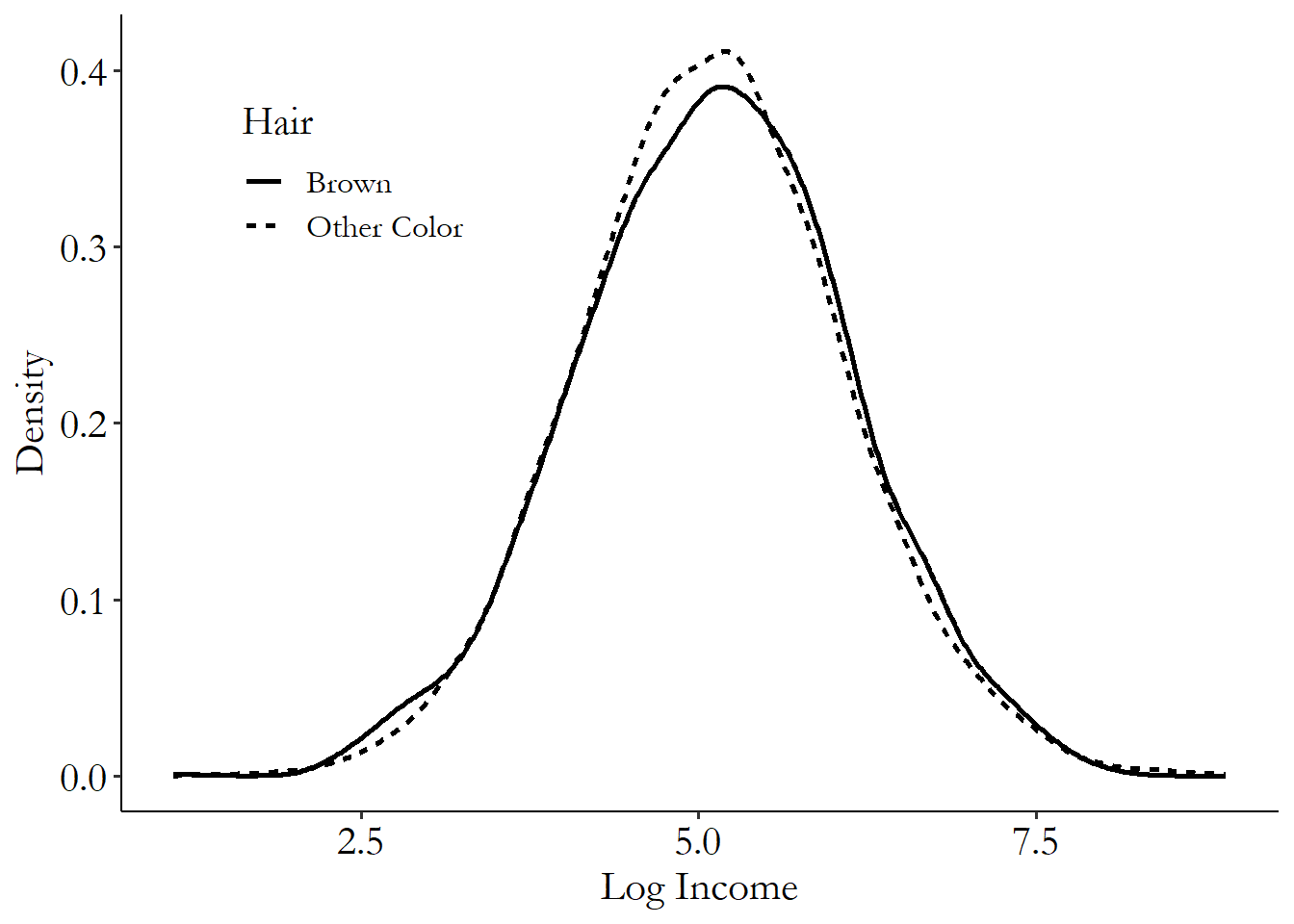
Table 5.1: Mean Income by Hair Color
| Hair | Log Income |
|---|---|
| Brown | 5.111 |
| Other Color | 5.095 |
Raw data. Data that has not been adjusted in any way.
What do we see in the raw data? We see that people with brown hair earn a little more. It’s hard to see in the figure, but in the table we can tell that they earn about .01 more in log terms, which means they earn about 1% more than people with other hair colors (see Chapter 3).
Uh-oh, that’s the wrong answer! We happen to know for a fact that brown hair gives you a 10% pay bump. But here in the data we see a 1% pay bump.
Where can we go from there in order to get the right answer? Not really anywhere. We have College information in our data, but without having any idea of how it fits into the DGP, we have no idea how to use it.
Now let’s bring in some of the knowledge that we have. Specifically let’s imagine we know everything about the DGP except the effect of brown hair on income.
If we know that it’s only non-college people who are dying their hair, and that College gives you a bump, we have some alternate explanations for our data. We don’t see much effect of brown hair because a whole lot of non-college people have brown hair, but those people don’t get the College wage bump, so it looks like brown hair doesn’t do much for you even though it does.
Knowing about the DGP also lets us figure out what we need to do to the data to get the right answer. In this DGP, we can notice that among college students, nobody is dying their hair, and so there’s no reason we can see why brown hair and income might be related except for brown hair giving us an income boost.
So in Table 5.2 we limit things just to college students. Now we see that brown-haired students get a bump of 13%. That’s not exactly 10% (randomness is a pest sometimes), but it’s a lot closer. And if we ran this little study a thousand times, on average we’d get 10% on the nose.
Table 5.2: Mean Income by Hair Color Among College Students
| Hair | Log Income |
|---|---|
| Brown | 5.340 |
| Other Color | 5.208 |
How the heck did we do that? We got the right answer (or close enough) in the end. We know that getting the right answer involves using information about the data generating process (DGP), and we did that. But what were we actually trying to accomplish by using that information, and how did we know how to use it? At this point I just sort of told you what to do. Not too helpful unless you’ve got me added as a contact in your phone.82 If you must call me with questions about identification, please limit it to business hours.
We can split this into two ideas, which we will cover in the next two sections.
Variation. How a variable changes from observation to observation.
The first is the idea of looking for variation. The DGP shows us all the different processes working behind the scenes that give us our data. But we’re only interested in part of that variation - in this case, it turned out to be the variation in income by hair color just among college students. How can we find the variation we need and focus just on that?
The second is the idea of identification. How can we use the DGP to be sure that the variation we’re digging out is the right variation? Figuring out what sorts of problems in the data you need to clear away - like how we noticed that the non-college students dying their hair was giving us problems - is the process of identification.
5.2 Where’s Your Variation?
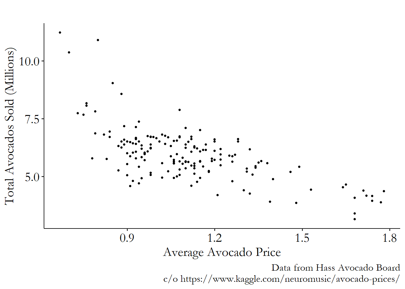
In a moment I’m going to show you a graph, Figure 5.2. This scatterplot graph shows, on the \(x\)-axis, the price of an avocado, and on the \(y\)-axis, the total number of avocados sold.83 Price is on the \(x\)-axis rather than the \(y\) for the purposes of aiding statistical thinking, and possibly also for the purpose of enraging several economists. Each point on the graph is the price and quantity of avocados sold in the state of California in a single week between January 2015 and March 2018.
I’m going to ask you to indulge me and spend a good long while looking at the graph. While you’re doing that, I want you to ask yourself a few questions:
- What conclusion can you draw from Figure 5.2? Think literally, as though you were a robot. Try not to see anything that isn’t really there.
- Now, think about the relationship between avocado prices and quantities more broadly. What kinds of research questions might we have about this relationship? For example, we might wonder what effect a 10% increase in price might have on the number of avocados people want to buy. Can you think of another research question?
- Can you answer your research question from Step 2 using Figure 5.2? Why or why not?
Figure 5.2: Weekly Sales of Avocados in California, Jan 2015-March 2018
All right - hopefully you’ve been able to come up with some answers to those questions. What do we have?
Negative relationship. When one variable is higher than normal, the other is generally lower than normal.
First, what do we literally see in Figure 5.2? We see that there’s clearly a negative relationship. What this tells us is that avocado sales tend to be lower in weeks where the price of avocados is high. Or, perhaps, prices tend to be higher in weeks where fewer avocados are sold. What we can see in the graph is the covariation or correlation between price and quantity of avocados.
That’s more or less it. That’s all. We might be tempted to say something like an increase in the price of avocados drives down sales. But that’s not actually on the graph! Or we might want to say that an increase in prices makes people demand fewer avocados, but that’s not on there either—any good economist will tell you that both supply and demand are part of what generates market prices and quantities, and we’ve got no way of pulling just the demand parts out yet. All we know is that quantities tend to be high when prices are low. We have no idea yet why that is.
Second, what research questions might we have about the relationship between price and quantity? There are a lot of things we could say here. Perhaps we’re interested in how price-sensitive consumers are - what is the effect of a price increase on the number of avocados people buy? Or heck, maybe we’re thinking about this the wrong way - maybe we should ask what is the effect of the number of avocados brought to market on the price that sellers choose to charge?84 There are, of course, many other questions to ask! What is the effect of the price on the number of avocados brought to market? What is the effect of the quantity sold one week on the number of avocados people will want to buy the next week? What is the effect of the price on the number of avocados that are brought to market but never sell? Each of these questions would require us to dig out a different part of the variation.
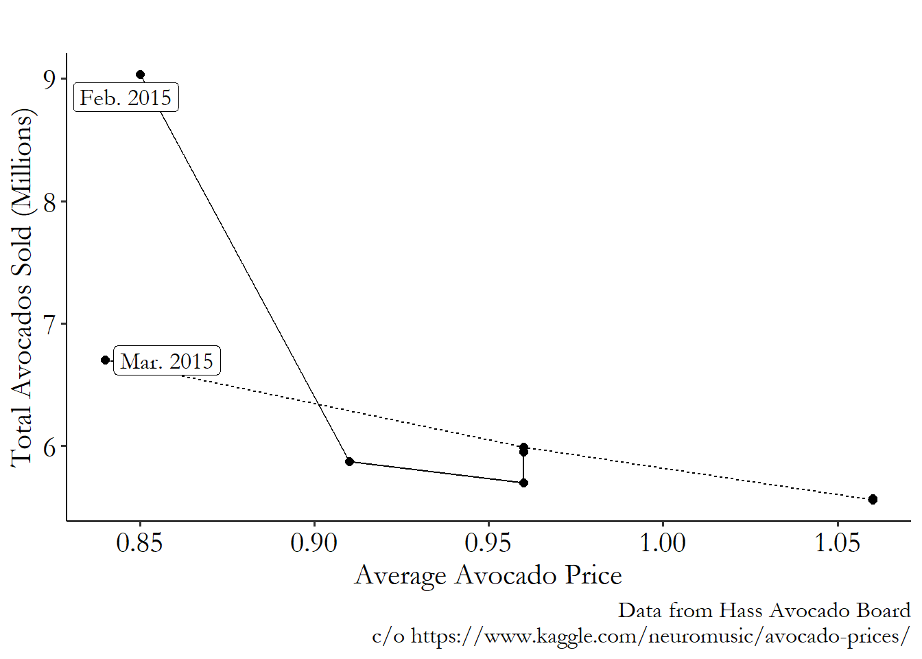
So, third, can we answer any of these questions by looking at the graph? Unfortunately, no.85 Unless your research question really was about what the correlation is. That question you can certainly answer. It’s not a bad question, either. The graph shows the covariation of price and quantity - how they move together or apart. But these variables move around for all sorts of reasons! Consider a simplified version of the graph, Figure 5.3. Figure 5.3 has only two points, from consecutive weeks.
Figure 5.3: Weekly Sales of Avocados in California, Jan 2015-Feb 2015
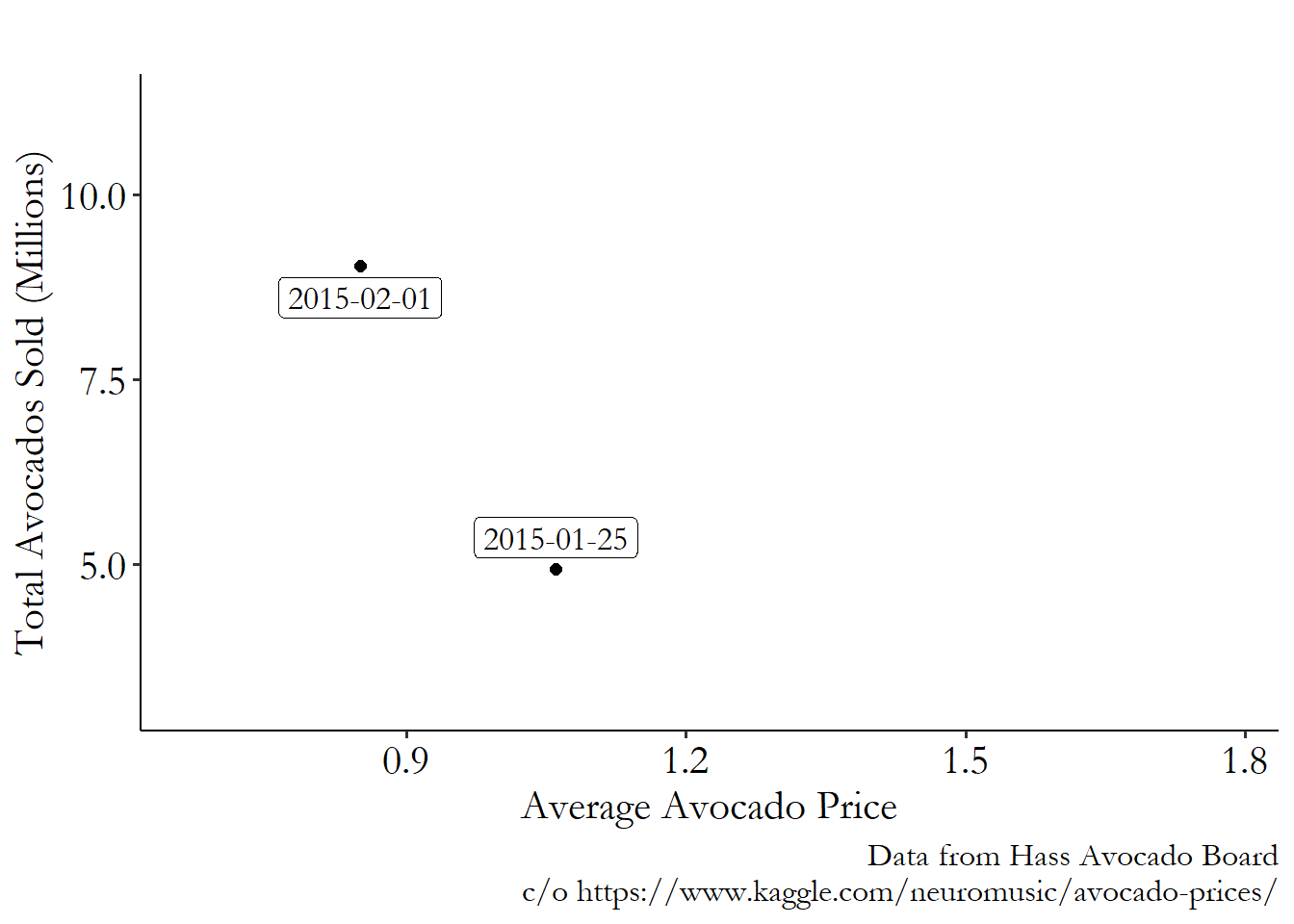
We can still see a negative relationship, which is the same as we saw in Figure 5.2. But why did price drop and quantity rise from January to February that year? Is it because a drop in price made people buy more? Is it because the market was flooded with avocados so people wouldn’t pay as much for them? Is it because the high price in January made suppliers bring way more avocados to market in February?
It’s probably a little bit of all of them. Variables move around for all sorts of reasons. Those reasons would be reflected in the data generating process (DGP). But when we have a research question in mind, we are usually only interested in one of those reasons.
So the task ahead of us is: how can we find the variation in the data that answers our question? The data as a whole is too messy - it varies for all sorts of reasons. But somewhere inside the data, our reason for variation is hiding. How can we get it out?
We have to ask what is the variation that we want to find? If we want to figure out what the effect of the price is on how many avocados people want to buy, then we want variation in people buying avocados (rather than people selling them) that is driven by changes in the price (rather than, say, avocados becoming less popular).86 Advanced readers may notice both the similarities and differences between this approach and the “ideal experiment” in Angrist and Pischke (2008Angrist, Joshua D., and Jörn-Steffen Pischke. 2008. Mostly Harmless Econometrics: An Empiricist’s Companion. Princeton University Press.).
As we discussed in the previous section, we’re going to be hopeless at doing this if we don’t know anything about the DGP. We need to use what we know about the DGP to learn a little more. So let’s make up some facts about where this data came from. Let’s imagine for a second that we know for a fact that at the beginning of each month, avocado suppliers make a plan for what avocado prices will be each week in that month, and never change their plans until the next month.
If that’s true, then the “suppliers set prices” and “suppliers set quantities” explanations only matter between months. The variation in price and quantity from week to week in the same month will isolate variation in people buying avocados and get rid of variation from people selling avocados. Further, because the price is set by the sellers, the variation in quantity we’re looking at can only be driven by changes in the price.
Our ability to find this answer is entirely based on that assumption we made about sellers making their choices between months. The reason I’ve made this particular assumption is that it helps us isolate (identify) only the variation on the part of consumers, conveniently getting rid of variation on the part of sellers and letting us just look at buyers.87 Would it be possible to identify what we want without this weird assumption? Sure! It’s kind of tricky though. Outcomes that are a combination of two separate systems working together - like buyers and sellers - are tricky to work with. But researchers manage to isolate variation in just one side, often using “instrumental variables,” which will be discussed more in Chapter 19. This assumption, which works so much magic for us, is entirely a fiction made up for the convenience of writing this book. Hopefully you will not find all assumptions made for the purposes of digging out variation to be convenient fictions. Some probably are.
By tossing out any variation between months, we’re digging through explanations that rely on that variation and tossing them out. Since sellers only change behavior between months (given our assumption), that explanation gets tossed out when we get rid of between-month variation, leaving us only with buyer behavior.
If we just look at changes within months, as in Figure 5.4, we can see that there’s still a negative relationship. Note that for each of the months, there’s a negative relationship, ignoring any differences between the months. So, given the data and what we know about how sellers operate, an increase in price does reduce how many avocados people want to buy.
Figure 5.4: Weekly Sales of Avocados in California, Feb 2015-Mar 2015
The task of figuring out how to answer our research question is really the task of figuring out where your variation is. It’s unlikely that the variation in the raw data answers the question you’re really interested in. So where is the variation that does answer your question? How can you find it and dig it out? What variation needs to be removed to unearth the good stuff underneath?
That process - finding where the variation you’re interested in is lurking and isolating just that part so you know that you’re answering your research question - is called identification.
5.3 Identification
Abel and Annie Vasquez woke up Tuesday morning to find that their faithful dog Rex was not at the foot of their bed as normal. Distraught, they ran through the house, calling his name, whistling, offering treats. Finally, one of them opened the front door, and there was Rex, sitting on the grass, wagging his tail. They brought him back inside.
“I keep telling you to latch the doggie door,” said Abel.
“He never uses that door anyway. I bet he jumps out that open window in the basement,” said Annie.
“Sure,” said Abel, rolling his eyes. That night, he made sure to latch the doggie door.
Abel and Annie Vasquez woke up Wednesday morning. The sun was warm, the smells of the automatic coffee machine had already reached their bedroom, and Rex was gone.
It didn’t take them long to find him this time, out on the lawn again, rolling in dew. A little patch of fur was getting rubbed raw - however he was getting out, it was clearly the same way every night.
That night, they latched the doggie door and double-bolted the back door. Thursday morning, Rex was gone.
Thursday night, they latched the doggie door, double-bolted the back door, and closed the blinds. Friday, Rex was gone.
Friday night, they latched the doggie door, double-bolted the back, closed the blinds, and blocked the air vent. Saturday morning Rex had eaten two butterflies before they found him outside.
“I’ve had enough of this,” said Abel. That night they locked and latched every door, closed every window, boarded up the chimney, sealed up the half-inch crack between the boards in the garage, plugged the drain in the tub, and gave Rex a very stern talking-to.
Sunday morning, Annie came downstairs to find Abel, distraught, sitting on the stoop and looking at his dog, who had once again escaped the house.
“I don’t understand… I closed off every possible way he could get out. Every crack, every crevice, every hole. Every possible exit was blocked. But there he is!”
Annie drank her coffee. “Oh, I opened the basement window back up before I went to bed. Told you that’s how he was getting out.”
The next night they left everything else open but closed the basement window. The next morning, finally, finally, finally, they woke up and Rex had stayed inside the whole night.
Identification is the process of figuring out what part of the variation in your data answers your research question. It’s called identification because we’ve ensured that our calculation identifies a single theoretical mechanism of interest. In other words, we’ve gotten past all the misleading clues and identified our culprit.
A research question takes us from theory to hypothesis, making sure that the hypothesis we’re testing will actually tell us something about the theory. Identification takes us from hypothesis to the data, making sure that we have a way of testing that hypothesis in the data, and not accidentally testing some other hypothesis instead.
Take Abel and Annie’s case. What do we see in the actual data? We see, on different nights, different parts of the house being sealed off, and we also see that Rex makes it outside each night. Annie’s research question is whether the basement window being open is what lets Rex out.
We - and Abel - know that there are plenty of ways to get out of the house. So this data alone doesn’t answer Annie’s research question. As Abel closes up more and more stuff, he is tossing out some of the variation. Every time he does, the number of places Rex could get out besides the window shrinks, so there are fewer and fewer ways that Annie could be wrong about the window, but there are still other explanations for how the dog got out.
But once we’ve closed up literally every other possible avenue out of the house, and the window is all that’s left, there’s only one conclusion to come to: the window being open is what let the dog out. This observation has identified an answer to our question, simply by closing off every other possible explanation.88 We can also see this identification process while watching magic tricks. A magician might show you their empty sleeves before producing a card out of nowhere. Why? They know there are plenty of ways they could produce a card (“it’s just hiding in their sleeve!”) and want to eliminate all the boring explanations they don’t want. They call this process of ruling out possible ways they did the trick “closing doors,” which coincidentally is very close to the “closing back doors” term we have for the same idea. We’ll get to that one in Chapter 8.
The process of closing off other possible explanations is also how we identify the answers to research questions in empirical studies.
Consider the avocado example in the previous section. Just like Abel and Annie considered all the ways their dog might be able to get out, we asked what are all the ways that prices and quantities might be related? Once we have an idea of what our DGP is, i.e., what are all the different ways that prices and quantities might be related, we will have a good idea of what work we need to do. Just like Abel and Annie closed off every possible avenue except the basement window, we closed off undesirable explanations by getting rid of between-month variation driven by sellers. The only way for price to affect quantity at that point is through the consumers.
Identification requires statistical procedures in order to properly get rid of the kinds of variation we don’t want. But just as important, it relies on theory and assumptions about the way that the world works in order to figure out what those undesirable explanations are, and which statistical procedures are necessary. Specifically, it relies on theory and assumptions about what the DGP looks like. We need to make a claim about what we already know in order to have any hopes of learning something new. In the avocado example, we used our knowledge about how markets work to realize that sellers might be setting price in response to the quantity - an alternate explanation we need to deal with. Then, we used an assumption about how sellers set prices to figure out how we can block out this alternate explanation by looking within-month just like Abel blocked up the chimney by using wood and nails.
It doesn’t instill a lot of confidence to acknowledge that we have to be making some assumptions in order to identify our answers, does it? But it is necessary. Imagine if Abel and Annie tried to figure out how the dog got out without any assumptions or knowledge about the data generating process. The list of alternate explanations they’d have to deal with would include “the dog can teleport,” “the universe is a hologram,” and “our walls have invisible holes only dogs can see.” They’d never come to a conclusion, and they’d be at serious risk of becoming philosophers.89 Granted, while we can’t avoid making assumptions we can try to avoid making unreasonable ones. “Dogs can’t teleport” seems fine. “Sellers make all choices at the beginning of the month and never change” is a bit iffy, at least without further information.
So then that’s our goal. If we want to identify the part of our data that gives the answer to our research question, we must:
- Using theory and what we already know about the world from previous studies or observations, paint the most accurate picture possible of what the DGP looks like
- Use that DGP to figure out the reasons our data might look the way it does that don’t answer our research question
- Find ways to block out those alternate reasons and so dig out the variation we need
This process is a lot more difficult than just “look at the data and see what it says.” But if we don’t go the extra mile of following these steps, we can end up with confusing, inconsistent, or just plain wrong results. Let’s see what happens when we don’t take identification quite seriously enough.
5.4 Alcohol and Mortality
If you are the type to pay attention to news articles with headlines beginning “A New Study Says…” you may find yourself deeply confused about the health effects of alcohol. Sometimes the study says that a few drinks a week is even healthier than none at all. Other studies find that alcohol is unsafe at any level. Or maybe it’s just wine that’s good for you?90 This same phenomenon plays out not just with alcohol but with pretty much every kind of food you can think of - chocolate, eggs, wheat. Great for us one month, deadly the next.
Let’s take a look at one major study, A. M. Wood et al. (2018Wood, Angela M., Stephen Kaptoge, Adam S. Butterworth, and 239 more. 2018. “Risk Thresholds for Alcohol Consumption: Combined Analysis of Individual-Participant Data for 599,912 Current Drinkers in 83 Prospective Studies.” The Lancet 391 (10129): 1513–23. https://doi.org/10.1016/S0140-6736(18)30134-X.), on the effects of alcohol on “all cause mortality” - basically, your chances of dying sooner. This study has more than 200 authors and studied the relationship between drinking and outcomes like mortality and cardiovascular disease among nearly 600,000 people. It was published in 2018 in the prominent medical journal The Lancet, and it has been used in discussions of how to set medical drinking guidelines, as in Connor and Hall (2018Connor, Jason, and Wayne Hall. 2018. “Thresholds for Safer Alcohol Use Might Need Lowering.” The Lancet 391 (10129): 1460–61.).
The study is very well-regarded! What it found is that there did not appear to be a benefit of small amounts of drinking. Further, it found that the amount of alcohol it took to start noticing increased risk for serious outcomes like mortality was at about 100 grams of alcohol per week, which is about a drink per day, and below current guidelines in some countries. Figure 5.5 shows the relationship they found between weekly alcohol consumption and the chances of mortality. Mortality starts to rise at around 100 grams of alcohol per week, and goes up sharply from there.
Figure 5.5: Alcohol Consumption and Mortality from Wood et al. (2018). Minor changes from original.
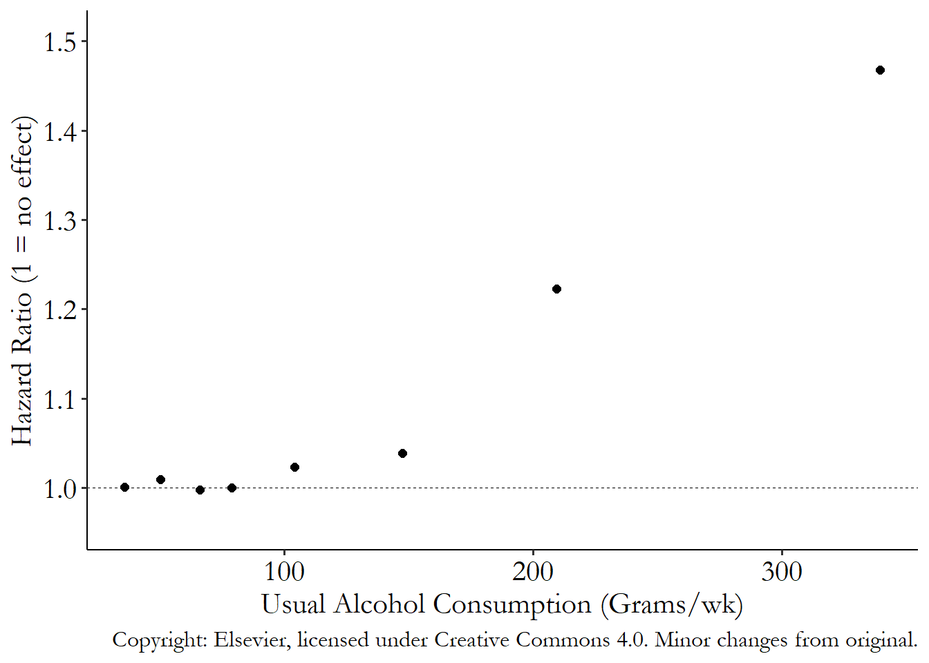
Hazard ratio or odds ratio. Not something we’ll be focusing a lot on in this book, but basically a proportional effect. So a 1.25 means you’re multiplying your hazard rate or odds (as appropriate) by 1.25.
We know from previous sections in this chapter that in order to make sense of the data we need to think carefully about the data generating process (DGP).
What is the DGP? What leads us to observe people drinking? What leads us to observe them dying? What reasons might there be for us to see an association between alcohol and mortality?
Pause here for a moment and try to list five things that would be a cause of someone drinking, or at least be related to drinking. Then, try to list five things that would be a cause of someone dying. Bonus if the same things end up on both lists.
Determinants of \(Y\). The set of variables that are part of the data generating process when \(Y\) is the outcome variable.
Did you come up with some determinants of drinking and mortality? There are certainly plenty of options. For example, a tendency to take more risks might lead someone to drink more, and may cause other things like smoking. So risk-taking is a cause of drinking, and because of that, smoking is related to drinking too. As for mortality, any one of a long list of bad-health indicators could cause mortality. So could something like smoking, risk-taking, or just working in a dangerous job!
You can see pretty immediately from this that anything that ends up on both lists is automatically going to be an “alternate explanation” for the results. Take smoking, for instance. If smokers are more likely to drink, and smoking increases mortality, then one reason for the relationship between drinking and mortality might just be that smokers tend to drink, and they also die earlier because of their smoking. Anything else that ends up on both lists is going to give us an alternate explanation.
There’s something else you may not have thought of - how about people who don’t drink at all? If drinking is very bad for you, surely non-drinkers would have very low mortality rates? Maybe, but keep the DGP in mind. Why don’t they drink? One reason people choose not to drink at all is because their health is too poor to handle it. Another reason is if they are recovering alcoholics. In these cases, we may actually see worse mortality for non-drinkers, but that relationship is almost certainly not because not-drinking is bad for them. That’s an alternate explanation too.
I’m going to bug you once again. Now that we’ve thought about it some more, I want you to pause and try to think of a few more reasons why we might see a relationship between alcohol and mortality other than alcohol being the cause of mortality. There’s no quiz,91 Unless you’re reading this book for a class and there is a quiz. but this is a very good habit to get into, both for the purposes of understanding the content in this book and for the purpose of trying to make sense of new studies and findings you read about.
Thankfully, the authors of the Woods et al. study did manage to deal with some of these alternate explanations. They were putting some thought into what the DGP looks like.
You may have noticed, for one, that Figure 5.5 actually doesn’t contain non-drinkers. They’ve been left out of the study because of the too-sick-to-drink and ex-alcoholic alternate explanations they want to block out. This is one reason why the study doesn’t find a positive effect of a little alcohol, while other studies do - some of those other studies leave in the non-drinkers (oops!).
The authors also use statistical adjustment to account for some other alternate explanations. They adjust for smoking, which was one thing we were concerned about, as well as age, gender, and a few health indicators like body mass index (BMI) and history of diabetes.
So they’re good, right? Well, not necessarily. Just because they’ve been able to account for some of the alternate explanations doesn’t mean they’ve accounted for all of them. After all, we mentioned risk-taking above. They adjusted for smoking, but surely risk-taking is going to matter for other reasons, and that’s not something they can easily measure. They took out non-drinkers who might not drink because they’re sick or ex-alcoholics. But that means they also took out non-drinkers who are neither of those things. And what if some very sick people just choose to drink less rather than not at all? There’s plenty more to think about, some of which you might have even noticed yourself while reading this chapter, that isn’t in their study. They clearly spent some time thinking about the DGP. But they might not have spent enough - or maybe they did spend enough but just weren’t realistically able to account for everything.
There are still some alternate explanations for their results that they couldn’t address. So it might be a little premature to take these results, despite the hundreds of thousands of people they examined, and use them to conclude that we have now identified the effects of alcohol on mortality.
If it feels like they did their part in addressing some of the alternate explanations and what’s left over feels trivial, keep in mind that these alternate explanations can lead us to very strange conclusions. Chris Auld (2018Auld, Chris. 2018. “Breaking News!” https://twitter.com/Chris_Auld/status/1035230771957485568.) read the study, and then took the same methods as in the original paper and used them to “prove” that drinking more causes you to become a man (see Figure 5.6).
Figure 5.6: Alcohol Consumption and Being a Man
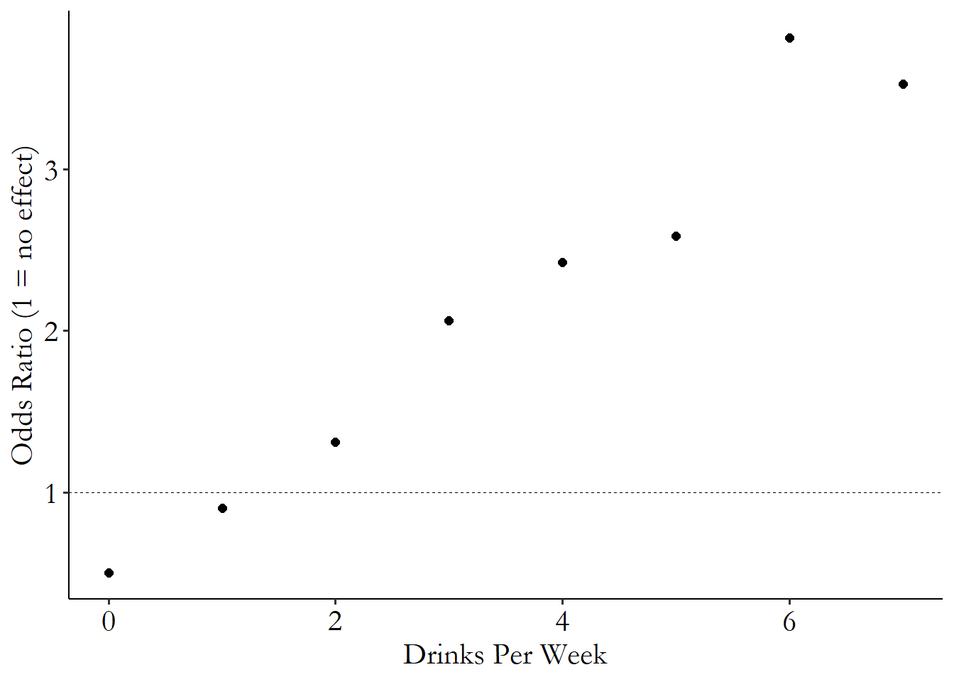
The idea that alcohol turns you into a male seems ridiculous, and in contrast it is pretty darn plausible that alcohol does really increase mortality. But if these methods can give us Figure 5.6, then even if there is really an effect of alcohol on mortality, how close do we think Figure 5.5 is to identifying that effect?
Is it, then, maybe a little concerning how much certainty there seems to be in the response to the study, and others like it, from the media and from medical authorities? The authors of this study have without a doubt found a very interesting relationship, and have addressed some alternate explanations for it. But have they identified the answer to the research question you’re really interested in - how drinking causes your health to change? That’s the question you would want to ask when making policy decisions like setting medical alcohol guidelines. Have they addressed all the necessary context? Is it even possible to do that?
5.5 Context and Omniscience
One thing that I hope this chapter has made clear is this: for most research questions, especially any questions that have a causal element to them, understanding context is incredibly important. If you don’t understand where your data came from, there’s no way that you’ll be able to block alternative explanations and identify the answer to your question.
In the words of Joshua Angrist and Alan Krueger (2001Angrist, Joshua D., and Alan B. Krueger. 2001. “Instrumental Variables and the Search for Identification: From Supply and Demand to Natural Experiments.” Journal of Economic Perspectives 15 (4): 69–85.),92 Copyright American Economic Association; reproduced with permission of the Journal of Economic Perspectives.
Here the challenges are not primarily technical in the sense of requiring new theorems or estimators. Rather, progress comes from detailed institutional knowledge and the careful investigation and quantification of the forces at work in a particular setting. Of course, such endeavors are not really new. They have always been at the heart of good empirical research.
They were specifically discussing identification using instrumental variables (see Chapter 19), but it’s true generally. Before attempting to answer a research question empirically, be sure to put in plenty of time understanding the context that the data came from and how things work there. Fill in as much of the data generating process (DGP) as you can! That’s going to be important both for interpreting your results properly, and for ensuring that there isn’t some equally-plausible explanation for your data that you can’t block out.
This means that there’s a lot of power in general understanding. So how should you start out designing your research project? By learning a lot of context. Read books about the environment you’re studying. Look at the documents describing how a policy was implemented. Read accounts and talk to people about how things actually work. Make sure you get the details right, because the details all show up in the part of the DGP you’re supposed to know.
This is either exciting news for you, or extraordinarily frustrating, depending on what kind of person you are.93 I will cop to finding this frustrating. What, you mean I have to figure out what reality is like to learn things about reality? I could prove way more fun things if we all just agreed the world should be how it is in my head.
It’s probably healthy to see this necessary reliance on context as both a great opportunity and also as a revelation about our limitations.
It’s a great opportunity because it means you get to learn a lot of stuff. And learning a lot of stuff is fun. If we didn’t like learning, we probably wouldn’t be interested in doing research in the first place. Also, learning about context may well be where we get the idea for the research question. As discussed in Chapter 2, a great way to come up with a research question is by studying an environment or setting and realizing that there’s something important about it that you don’t know. If that’s what you’re doing, by the time you have a research question, the contextual-learning part will already be done.
That learning may also help you figure out how to block off alternate explanations. Someone with a research question about gravity who has no idea about physics might be able to guess that magic isn’t responsible for planetary movement. But someone who really studies how planets move will be able to do the appropriate calculations to show that it’s not just momentum explaining how they move - you need gravity, too.
However, the need for context also reveals our limitations. If we can only really answer our research questions when we understand the context very well, then our only successful projects will tend to be in areas that we already mostly understand. Boring! What about those wild, out-there frontiers where nobody understands anything? Surely it’s not a good idea to just ignore them. After all, even if we will have trouble pinning down an exact answer, some questions, like the effects of alcohol on mortality, are too important to ignore completely.
We shouldn’t ignore those out-there exciting realms for research. But the need for context means that we should be prepared for our results to be more questionable, more prone to alternate explanations, more “exploratory.” This is just plain intellectual humility, and it’s a good thing. Knowing less means we can prove less. Forgetting that can lead us to make wild claims that end up being wrong when we know more.
You can see this pretty much any time anything new is introduced to society - novels, trains, universal voting, television, the Internet, video games. When these things are new, we don’t know how they fit into the DGP since we haven’t seen them produce any data. But that doesn’t stop people from producing wild claims about how they will save/destroy all of society. And there’s never a shortage of questionably performed research proving both the devotees and the skeptics correct, only for it all to be overturned as we learn more about how these things work.
Even at a smaller scale, the need for more context can be stymieing. Forget trying to study the effects of flying cars or space aliens. How can we even have enough context to study the effect of avocado prices on avocados sold? You can spend years studying the topic and become the world’s leading expert, and you’ll still never know everything about it. In order to truly be able to see all the alternative explanations for your data and truly understand all the underlying tantalizing-but-invisible laws, it’s almost like you need to be omniscient. How can you be sure there aren’t any holes left in your research?
Well… you can’t!
Sorry.
No research project is perfect. All we can hope to do is:
- Learn what we can about the context so that we don’t miss any hugely important part of the DGP
- Be careful to acknowledge what assumptions we’re making, and think about how they might be wrong
- Try to spot gaps in our knowledge about the DGP, and make some realistic guesses about what might be in that gap
- Not aim for perfection, but aim for getting as close as we can
If we try to be omniscient, we’ll always fail. So there’s no point in that. But there is a point in trying to be useful. For that we simply need to learn what we can, work carefully, and try to make our errors small ones.
Page built: 2025-10-17 using R version 4.5.0 (2025-04-11 ucrt)